EMPANADA Guide

To begin, I would recommend that one starts with the official empanada guidebooks as located here: https://empanada.readthedocs.io/en/latest/empanada-napari.html

Much of what I will be talking about is found here, but I will go over a few caveats that I've found in the process and try to explain the segmentation workflow in a step by step process.

Opening the software:

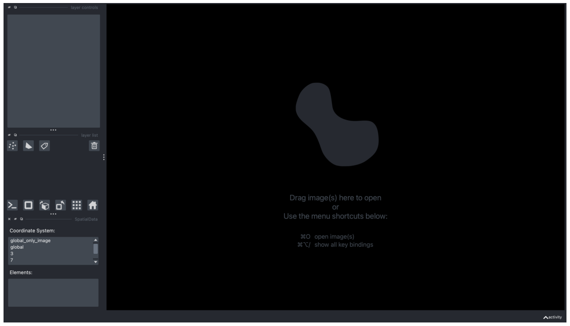
First, ensure that you have the software installed. This is best done by using the anaconda package manager. Through this, you can install NAPARI, the image viewer that EMPANADA runs. Once those are installed, you will have to activate the instance through the miniconda terminal by typing "napari". Note that if you made a virtual environment for running napari in, you will first have to run the command "conda activate [NAME OF INSTANCE]", with [NAME OF INSTANCE] replaced to what you named your virtual environment. Creating a virtual environment makes keeping track of dependencies easy, as NAPARI requires an older version of python than the machine may run. You should then be greeted by an interface that looks like this:

Loading a model:

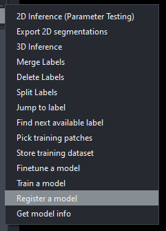
By default, Emapanda comes with it's own model, MitoNet. As you can guess it is used for identifying mitochondria. The IGB core staff have also developed a primitive model for identifying the cores of myelin sheaths. You can tenatively find this model in the core server at \\core-server.igb.illinois.edu\groups\core\core server\shared\2023\empanada-tests\mylin_sheaths\tuned_data\mylin_test\unknown under the file name PanopticDeepLabPR_Mylinium.pth. With the empanada plugin loaded, go to the "Register a model" option, then follow this path and click on the proper .pth model to register it into the program.

Loading an image:

There are three methods of opening images in the napari image viewer. You can open them as a single image, a stack, or a folder. The image option will allow you to select a single image, whereas the stack and folder option will let you either select a certain subsection of the folder, or the entire folder. Be careful, napari will not verify your selections, so make sure you are only selecting images.

Running an image segmentation:

There are two options to run an instance of a segmentation that may seem similar, but do slightly different tasks. The 2D image segmentation program is simpler than its 3D counterpart. Each layer of image is taken into account separately than in the 3D version. This means that sometimes layers will be over segmented in the 2D version meaning that the program tries to give the same part of an image a label more than once. This typically does not happen in the 3D version. The tradeoff is that the 2D version is often faster than the 3D version, so it is advisable that one use it for basic parameter testing and other tasks, and then when you have verified your results, bring it into the 3D segmentation version.

Here are some of the options you will see and what they all mean:

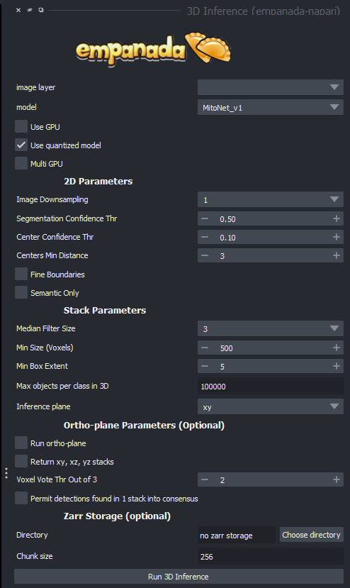
NOTE: Raw images from the microscopes in the lab will often be 32bit TIFFs, these will not work in empanada! You must convert them into either 16 bit or 8 bit tiffs for segmentation to not throw an error!

image layer: the current image set you are working on.

model: which segmentation model you are running

use gpu: use the graphical processing unit (GPU) for faster processing (our machine are equipped with very good GPUs, so you will almost always want to run this)

use quantized model: enables better performance for cpu models, be careful, this operation has precedence over GPU mode!

multi GPU: use multiple GPUs, our machines don't have them, so this option is meaningless

Image downsampling: If your image is oversampling, a trick could be this option, which basically scales down your image by a factor of the number you choose. This can be helpful for oversampling, but watch out for smaller segments getting lost.

Segmentation confidence thr(eshhold): Tells the computer how confident you'd like it to be in its selection of segments. Higher confidence means less segments, lower confidence means more, but better chances for false positives.

Center confidence thr(eshhold): This tells the computer how confident to be in where the center of the desired target is, it is not as important as the segmentation confidence, but can sometimes help prevent segmentation leaks if cells are tightly packed.

Fine boundaries: Much like the previous option, helps prevent segmentation leakage into other cells/organelles if your boundaries aren't well defined.

Semantic only: Only judges a segmentation by its shape, not any of its details, I generally wouldn't recommend this option.

(These next parameters are exclusive to the 3D version of the software)

Median Filter Size: the number of image layers to apply a median filter to, which smooths out the image in order to make semantic segmentation easier, but may distort tiny details that could be critical to detection.

Min Size (Voxels): The smallest object that is allowed to be segmented instead of filtered out as noise.

Min Box Extent: The size of a minimum bounding box to make sure there aren't an long spaghetti strand like segments that are often useless.

Max objects per class (also found in 2D): maximum segmentations per image classifier if a model segments more than one type.

Inference plane: which plane to go through as your microscope did to get a proper 3D stack, xy is often sufficient.

Run ortho plane: This is the function that turns your AI segmentation into 3D models. NOTE: This does not work with our current microscopes as almost all of them are anisotropic!

Return xy, xz, yz stacks: Return every stack that the software generates in the 3 possible planes.

Voxel vote thr out of 3: this is the amount of layers that a segmentation must be present in to be displayed in the ortho plane.

Note that the tick box "permit detections found in 1 stack consensus" is the equivalent of setting the top option to 1.

Zarr storage is useful if your machine doesn't have enough ram to work with your image sets (typically workstation machines have anywhere from 8-256, if your image set is bigger than this, you'll likely want to use it), it stores the segmentations temporarily on disk.

Directory: the directory where these temporary stacks will be stored

Chunk size: how big you want your temporary images to be, as they stay saved on disk and can be extracted if desired.

Training a model:

As a researcher or core staff assistant, you will find situations other than myelin sheaths and mitochondria that you or others will want segmented. This will require two key components. The first is training data, and the second is segmented data corresponding to the desired organelle of the training data. Once you have these two things, you can begin training a model. Empanada requires a certain directory layout for the data, you can achieve this in an easy manner by using the store dataset tool. Just specify the images and the segmentations and which directory you'd like to output this to.

Next thing is to do is to run the "train model" module, which looks like this:

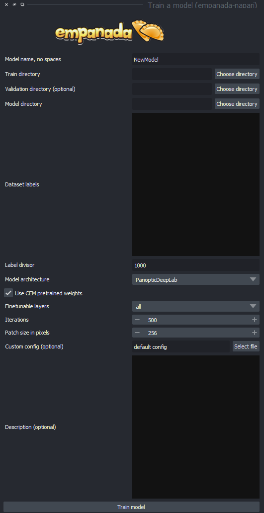
The options for this are as follows:

Model name: the name of the model you wish to create, make sure it is descriptive of the organelle you are targeting to avoid confusion.

Train directory: The directory of the unsegmented images, NOTE that this should be the top level above the folder which contains the folders for the properly formatted images and segments if done with the store database command.

Validation directory: The directory in which the segmentations are contains. This says it is optional, but note that the segmentations are not optional in themselves, but rather this option should be used if the segmentation directory lives in a separate directory from the images, if no input is made, the program will use the same directory from the train directory.

Dataset labels: When segmenting your data, you will have be able to mark different types of organelles in your cell. These should be marked with labels that fit into a certain section of label numbers. For instance, you could mark mitochondria in the 1000s, golgi complex in the 2000s and so on. How you define these ranges is up to you, but make sure you mark the boundary in the label divisor option. In this option, you will have to specify each group of segmented organelle (this can be a simple list of 1 through the amount of groups, this is just to tell the computer which groups are different), the name, and segmentation type, semantic or instance. Semantic segmentation is solely based on the shape of the object, but instance segmentation is based on the shape, placement, and details, and as such is generally more useful.

Here is an example of a proper format:

1,golgi,semantic

2,ER,instance

3,mitochondira,instance

Model architecture: Which architecture you want to use for training your model.

Fine tunable layers: Denotes which stages in the architecture to apply fine tuning to. This should generally be set to "All".

Iterations: How many times the model should be trained on the dataset. The default 500 generally gives the best results, but if you want to shorten the amount of training time (this could easily be tens of hours), then reducing the iterations will help.

Patch size in pixels: The general size of segmentations in pixels, must be divisible by 16.

Custom config: You can use this to specify a config file with all the options pre-set. May be useful if you are trying to train many similar models for comparisons.

Description: A free text box in which you can tell any future users any details about your model, such as what it was trained on, best use parameters, and possible weaknesses of your model.

Once this is all set up, you should have to wait somewhere between 10 and 20+ hours depending on how big your image set is. After that, you should see a .pth file appear in wherever you specified your target directory to be. If your model did not automatically load into the software, you can use the register a model program mentioned previously.

Finetuning a model:

Finetuning a model is normally meant to clean up segmentation rather than add new data to your model. You can use this if you want to simply refine your model, as it will take much less time to finetune data you already have versus add new data and regenerate your model. Normally the workflow for this is as follows: Generate segmentation on a sample. Clean up any errors in the segmentation. Use the "pick patches" tool to select 16 or more (software limitation) segmentations to feed the computer. Store them as a database. Run the database through the finetuning tool. The finetuner has almost all of the same options as the trainer, so I will not repeat my word in this section, simply check the train a model documentation.

Other tools:

The software suite consists of a number of other tools that are for ease of use. These are not critical to the training or segmentation process, so I will only cover these tools briefly.

Merge labels:

This tool merges two of the layers on the left hand side of the screen (don't get this confused with merging segments, which can simply be done with the paint bucket tool). To use this, you will need to go to your stack of choice. From there you will mark the layers that you want merged with the point tool.

Delete labels:

Much like the merge labels tools, this one functions quite similarly, select the stack you'd like to delete from, use the point layers to select which layers from the stack should be subject to deletion.

Split labels:

This will put any segmentations within a certain range of the point placed on a separate layer from the currently selected layer, you will need your points layer and your stack as arguments once again. You can also adjust a slider to tell the computer what radius from the point should be considered.

Jump to label:

Given a label ID, jump directly to it. Though it may be easier to simply use the in built NAPARI arrow buttons at the top left to simply cycle through which label you want to interact with.