# MINFLUX
Molecular resolution in 2D and 3D
# Introduction
#### **Minflux is a florescence imaging and tracking technique using a 2D doughnut or 3D bottle beam to localize switchable fluorophores to single digit nanometer resolution.**
Expanding on this
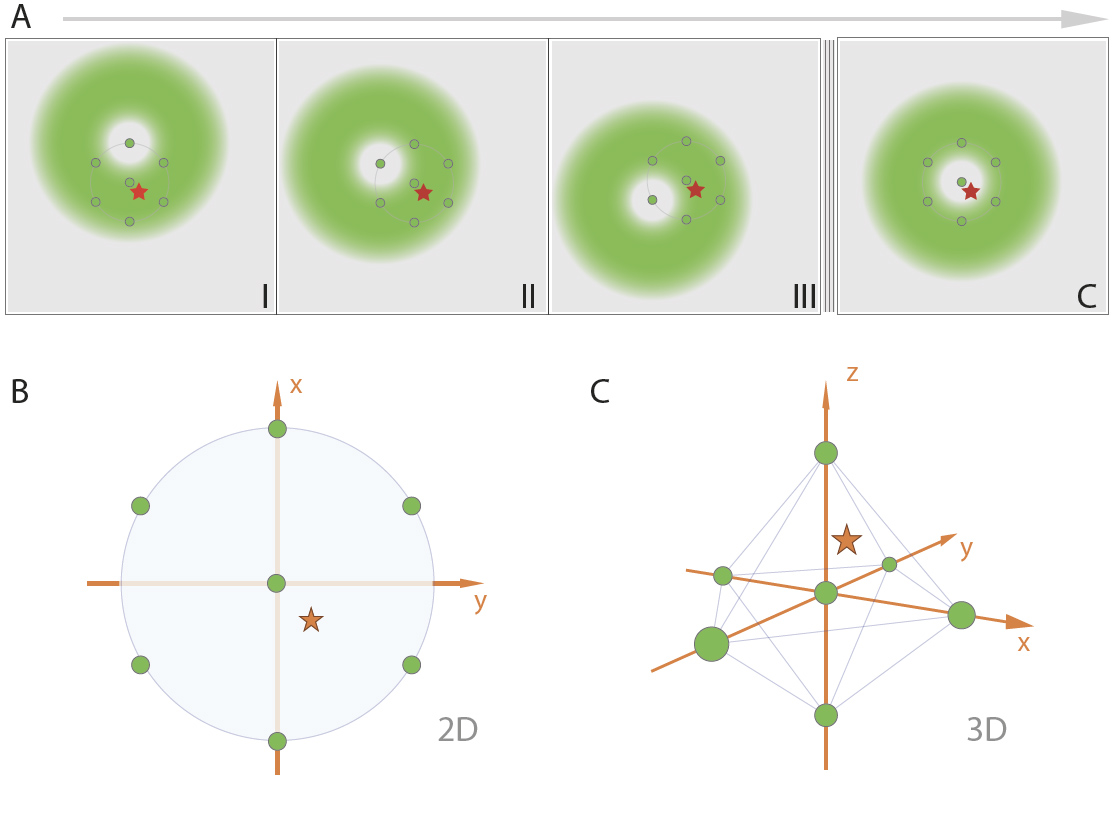
Minflux turns on fluorophores using a 405 laser. This allows the microscopist to control the number of active fluorophores and eliminates the situation where two active fluorophores are close together.
Minflux scans a sample with a doughnut shaped beam when an activated fluorophore is found (red star) in a field of fluorophores in a dark state (circles) the center of the excitation doughnut (green spot) moves in a hexagonal pattern 2D or octahedral pattern in 3D with a spherical excitation pattern, to determine the location of the fluorophore. The search pattern is minimized sequential.
[](https://www-app.igb.illinois.edu/core-docs/uploads/images/gallery/2022-07/image-1659038514583.png)
From Minflux unrivaled resolution Abberior
#### **Light Path**
[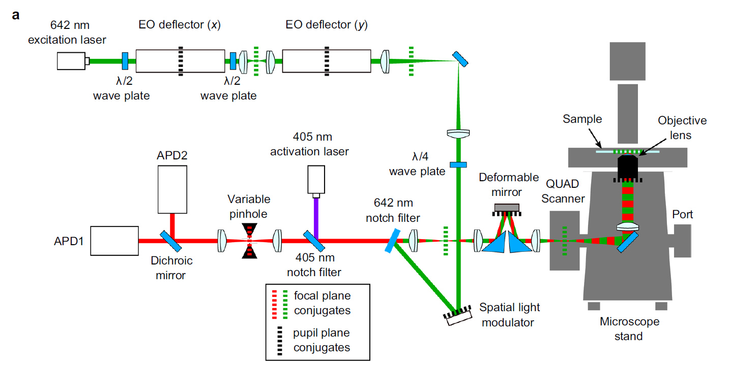](https://www-app.igb.illinois.edu/core-docs/uploads/images/gallery/2022-07/image-1659038580252.png)
#### **Sample preparation**
Cells are seeded on 18mm glass coverslips (No 1.5 or 1.5H); or chambered coverslips (no plastics cover slips). Fixation is done as usual (Formaldehyde or Methanol).
Minflux uses labeling techniques developed for dSTORM, so this means that Alexa fluor 647 is common. along with an oxygen scavenging GLOX buffer. β-mercaptoethylamine (MEA) is used as a blinking agent. Fiducials are also used.
Sample mounting and imaging buffers. For the sample stabilization during MINFLUX measurements, gold nanorods (A12-40-980-CTAB-DIH-1-25, Nanopartz Inc.) are used as fiducials. In brief, an undiluted dispersion of the nanorods is applied to the ready-made samples. Before mounting the samples in imaging buffer, the coverslips are rinsed several times with phosphate buffered
saline (PBS) to remove unbound nanorods. For MINFLUX imaging of samples labeled with Alexa Fluor 647, GLOX buffer (50mM TRIS/HCl, 10mM NaCl, 10% (w/v) Glucose, pH 8.0, 64 μg/ml catalase, 0.4 mg/ml glucose oxidase, 10–25mM MEA) is used. Samples are sealed with twinsil (picodent). **Ref 1**
#### **Labeling Dyes**
Live Cell Imaging (PALM) and Single Molecule Tracking:
\- Photo-switchable Organic Dyes/ Proteins, e.g., Janelia Fluor 549 or 646 dyes (Tocris)
\- Photoconvertible Oganic Dyes/ Proteins, e.g., mMaple (plasmids sold by Allele Biotechnology)
Fixed Cell Imaging (dSTORM):
-Carbocyanine dyes (sCy, ATTO, Alexa Fluor or Flux dyes may be used). Various dyes excited at 640 nm, such as Alexa Fluor 647, CF660C, CF680 or sCy5 can be used. Best Dye: Alexa 647 or Flux 647 for one color and sCy5 + CF680 or Flux 640 + Flux 680 (recommended) for 2 color-imaging.
Intracellular/Surface Live Cell Imaging (dSTORM):
\- SNAP, CLIP or Halo-tags for single color live cell imaging
\- SNAP & CLIP-tags for 2-color
\- SNAP & Halo-tags for 2-color (preferred if already in cell line)
\- Nanobodies (Proteintech)
No DAPI or Hoechst staining in sample. Labeling density should be very low (dilute antibodies 1:500 to 1:1000) to avoid over-labeling.
Background labelling: there should be no background.
\- increase blocking steps & times
\- increase washing steps & times
\- reduce antibody concentrations
#### **Stabilization**
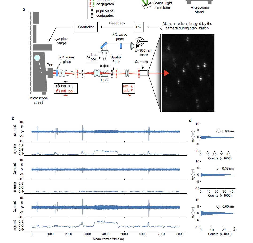
Sub nanometer stabilization is required to measure the location of a fluorophore to nm resolution. This system preforms to 0.39nm in x and y and 0.6nm in Z. This performance is impressive since 980nm light is used.
980nm light (easily passes through tissue) passes through a half wave plate to rotate polarization and then through a polarizing beam splitter and relay lens to focus on the back aperture of the lens. A quarter wave plate changes the linearly polarized light to right-handed circularly polarized light. Reflected left-handed circularly polarized light changes to vertically polarized light and passes through the polarizing beam splitter, a spacial filter and travels to the camera. The spacial filter removes low spacial frequency information from the image.
[](https://www-app.igb.illinois.edu/core-docs/uploads/images/gallery/2022-07/image-1659038909153.png)
figure from Ref 1
[](https://www-app.igb.illinois.edu/core-docs/uploads/images/gallery/2022-07/image-1659038939789.png)
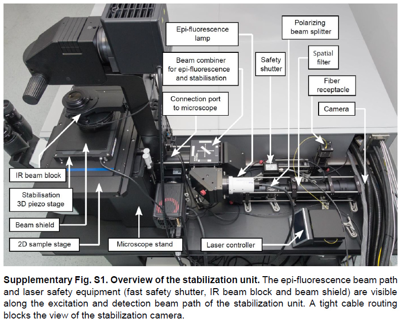
from supplement
gold nanorods rotating force: https://www.osapublishing.org/oe/fulltext.cfm?uri=oe-22-21-26005&id=303075
References
1 Schmidt R., et al. (2021) MINFLUX nanometer-scale 3D imaging and microsecond-range tracking on a common fluorescence microscope. Nat Commun., 12(1):1478.
2 Balzarotti, F. , et al. (2017). Nanometer resolution imaging and tracking of fluorescent molecules with minimal photon fluxes. Science, 355(6325), 606–612.
# Separating two signal based on dcr (detector channel ratio) in paraview
**Goal:**
- to separate signal form 2 detectors (CY5 near vs CY5 far), especially when you have two dyes for example AF640 and AF680
1\. Open image in **Imspector**
2\. **Minflux Data Panel** → Data source: it is usually **None**, so you must select data source that you want to view in Paraview.
3\. **Minflux Data Panel** → **Launch Paraview [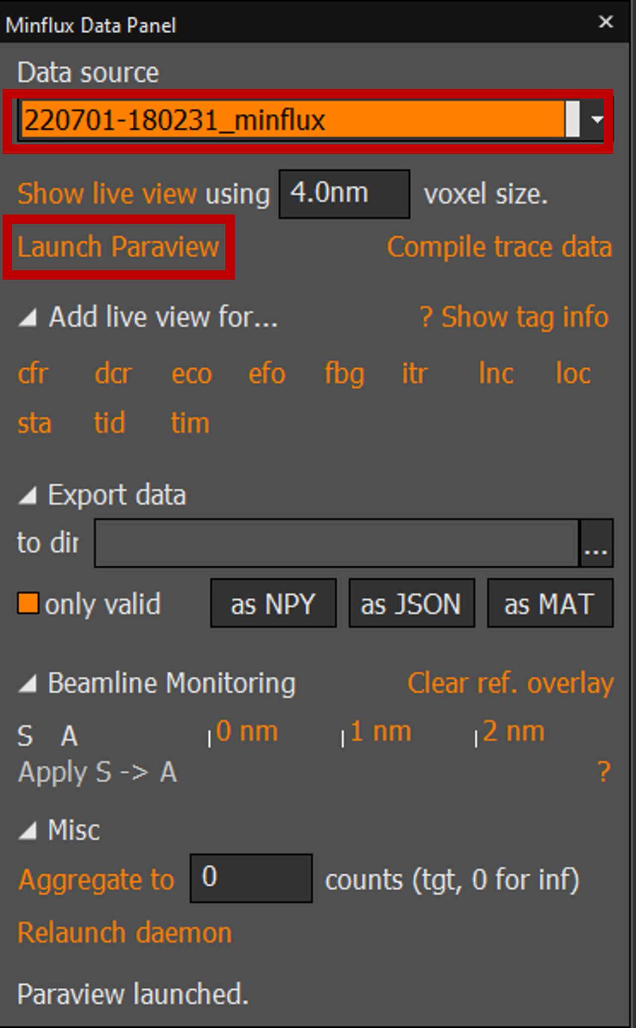](https://www-app.igb.illinois.edu/core-docs/uploads/images/gallery/2022-07/picture1.png)**
4\. in **Paraview** → under localization tab →select coloring to dcr (detector channel ratio)
[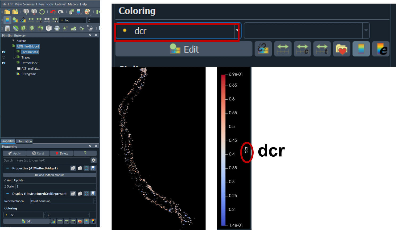](https://www-app.igb.illinois.edu/core-docs/uploads/images/gallery/2022-07/picture10.png)
5\. in **Paraview** → under localization tab → click right add filter → data analysis →histogram →**select input array** dcr → change bin count to 100 → press apply [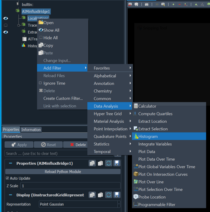](https://www-app.igb.illinois.edu/core-docs/uploads/images/gallery/2022-07/picture3.png)
[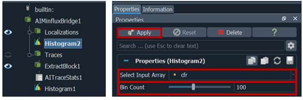](https://www-app.igb.illinois.edu/core-docs/uploads/images/gallery/2022-07/ss4.png)
6. From histogram plot we can see two peaks from CY near and CY far detector, we can separate the two channels for example here we want to discard dcr value from 0.32 to 0.36 [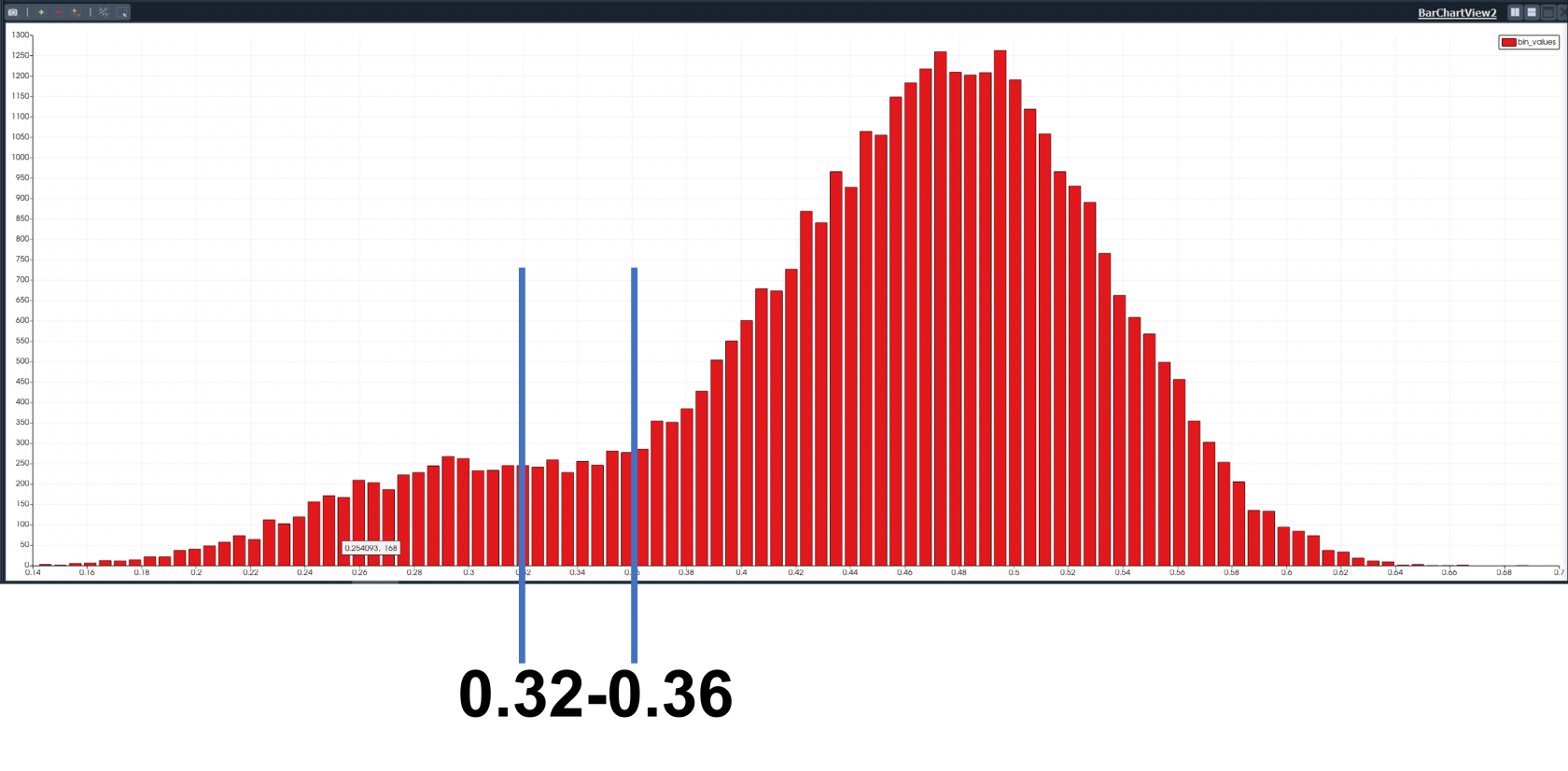](https://www-app.igb.illinois.edu/core-docs/uploads/images/gallery/2022-07/picture6.png)
7. localizations tab: you will see color map editor or rainbow icon (edit color map) to show the color map editor [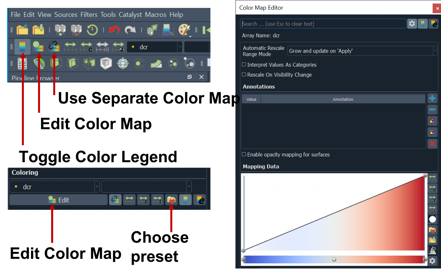](https://www-app.igb.illinois.edu/core-docs/uploads/images/gallery/2022-07/picture7.png)
8. **Choose Preset** to change color map you want to use for example **cold and hot** and click apply [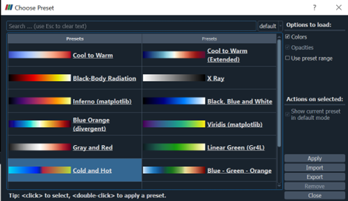](https://www-app.igb.illinois.edu/core-docs/uploads/images/gallery/2022-07/ss7.png)
9\. drag the color map **(A)** on the left side up **(B)→** we want to discard dcr value from 0.32 to 0.36 we will set this to black color: set the left circle the lowest dcr value 0.32 (enter the value on Data and click enter) and the right circle to 0.36 → make another two circles 0.32 and 0.36 on the middle circle double click on the center of circle then select color: choose black, repeat for the left circle for example select cyan HTML#00e9e9, and for the right circle select orange HTML #ff8206 [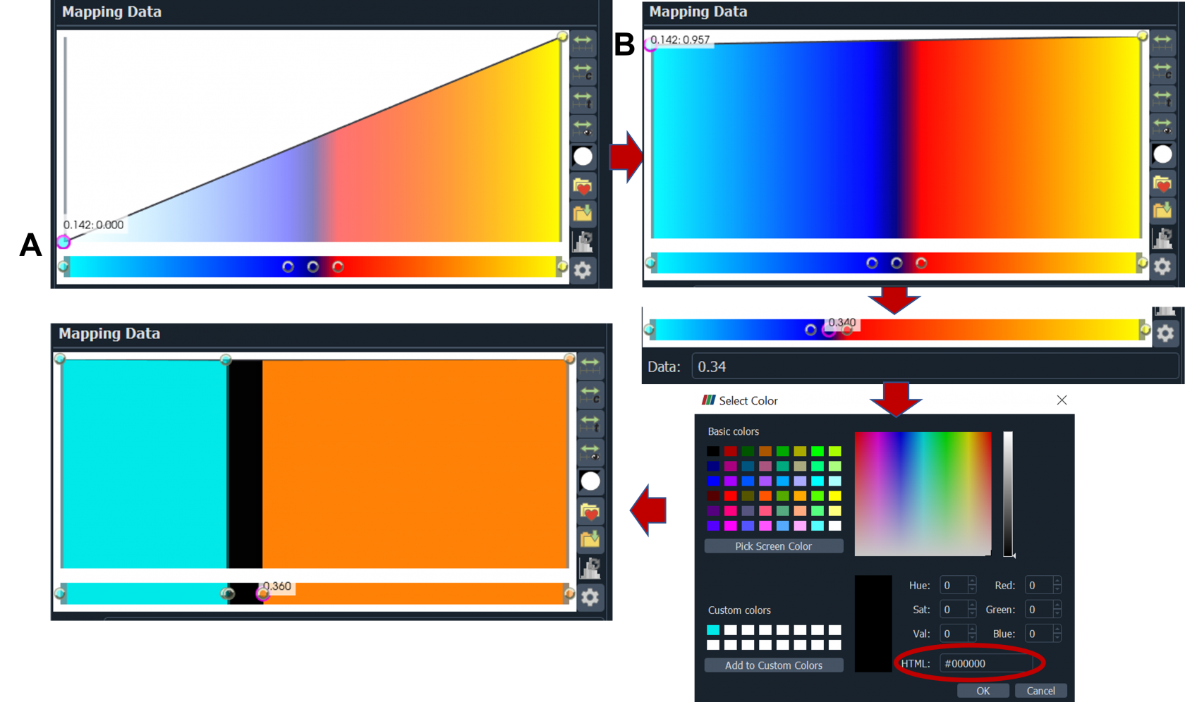](https://www-app.igb.illinois.edu/core-docs/uploads/images/gallery/2022-07/picture11.png)
10\. Signal with dcr value from 0.14 to 0.32 in cyan and dcr value of from 0.36 to 0.7 in orange [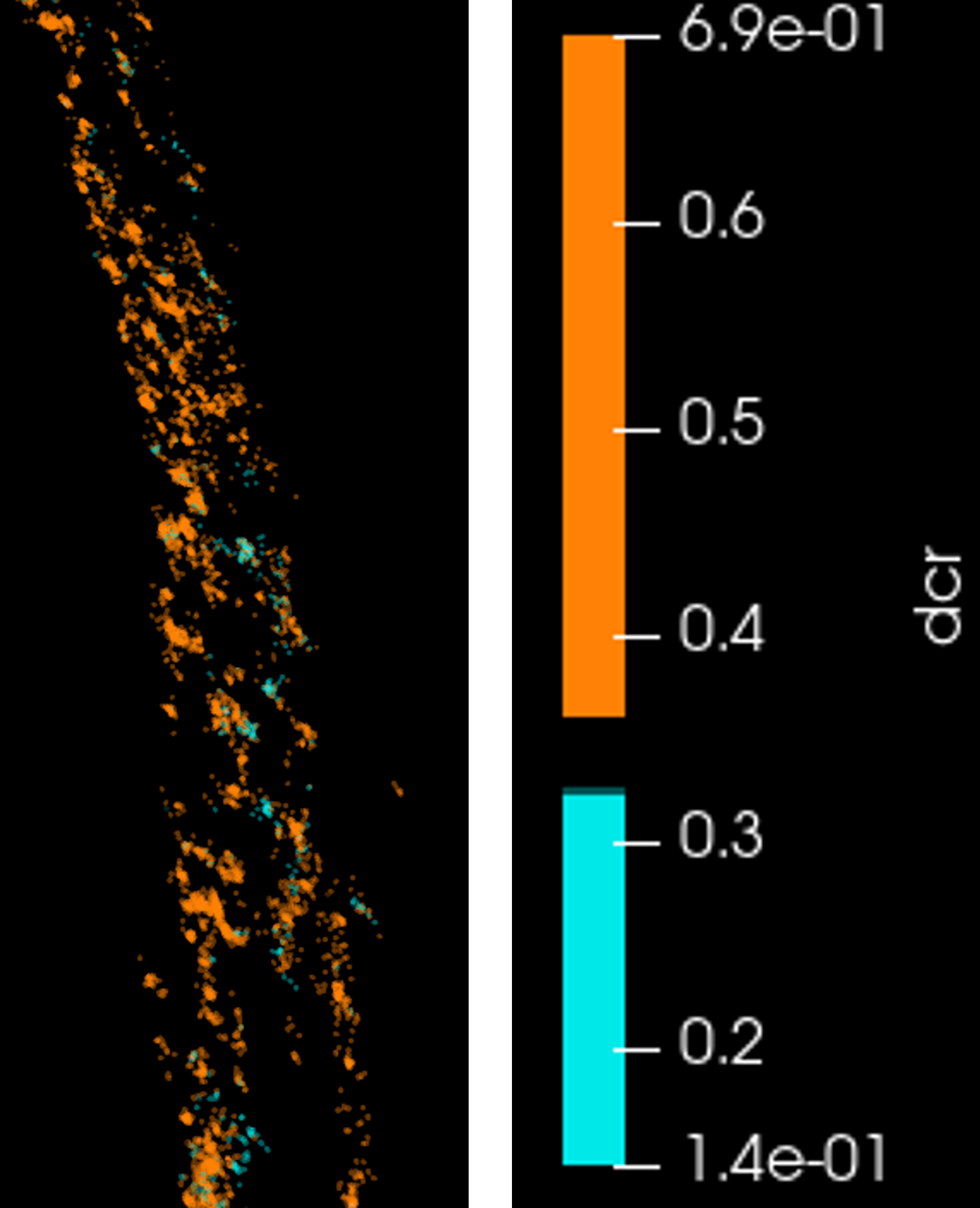](https://www-app.igb.illinois.edu/core-docs/uploads/images/gallery/2022-07/picture9.png)
# Superimpose images in Imspector
**Goal:**
- Superimpose confocal images
- Superimpose confocal image with Minflux image
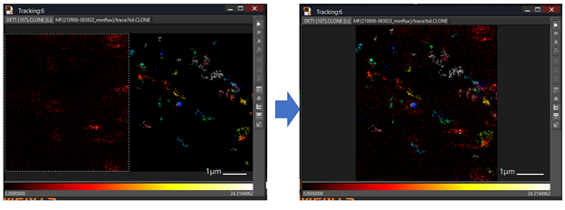
Note: Images can be combined if they have the same length and the same pixel size. In general, the pixel size of the Minflux image usually is much bigger than confocal image. As a result, we need to do image interpolation to make sure the pixel size of the two images is the same. Length and pixel size of an image can be checked using **change Stack Size** by pressing **CTRL T**. msr file can be opened in image J.
***Step by Step Superimpose images:***
1. Example: combine a confocal image and a minflux image, both images have the same length however the pixel size are different. [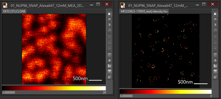](https://www-app.igb.illinois.edu/core-docs/uploads/images/gallery/2022-07/image1.png)
2. Select an image and press **Ctrl T[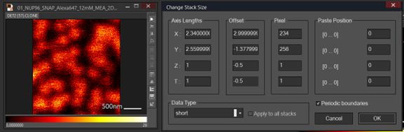](https://www-app.igb.illinois.edu/core-docs/uploads/images/gallery/2022-07/image2.png)**[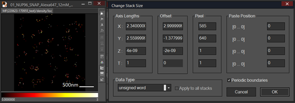](https://www-app.igb.illinois.edu/core-docs/uploads/images/gallery/2022-07/image3.png)
3. Change the pixel size of a confocal image to match the minflux image: go to **Analysis** and **Interpolation**, Change the resolution of confocal image to pixel size of minflux image, choose **result format** to **float** and press Now, we have similar length and pixel images. [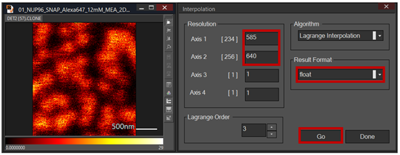](https://www-app.igb.illinois.edu/core-docs/uploads/images/gallery/2022-07/image4.png)
4. Choose new window [](https://www-app.igb.illinois.edu/core-docs/uploads/images/gallery/2022-07/image5.png)
5. Copy the image (Ctrl C or press **A**) and paste (ctrl V or press **B**) into the new window. When you paste the second image, warning appear “pixel dimension mismatch ignore and paste?”, select yes [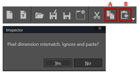](https://www-app.igb.illinois.edu/core-docs/uploads/images/gallery/2022-07/imag6.png) [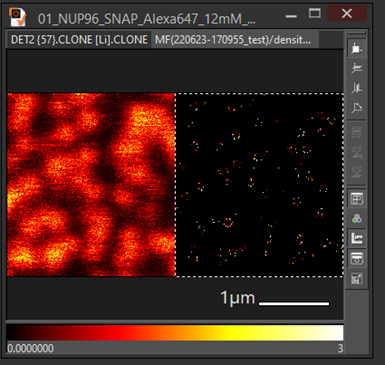](https://www-app.igb.illinois.edu/core-docs/uploads/images/gallery/2022-07/image7.png)
6. Change the color map or each image or choose RGBize then superimpose the image using **gallery mode** or **Ctrl G[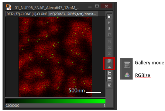](https://www-app.igb.illinois.edu/core-docs/uploads/images/gallery/2022-07/image8.png)***An example superimposes confocal image with tracking image:*
[](https://www-app.igb.illinois.edu/core-docs/uploads/images/gallery/2022-07/image9.png)
# Tracking in ParaView
Goal: how to analysis tracking data in paraview
1 **Imspector**: open your image in Imspector
[](https://www-app.igb.illinois.edu/core-docs/uploads/images/gallery/2022-08/tracking1.png)
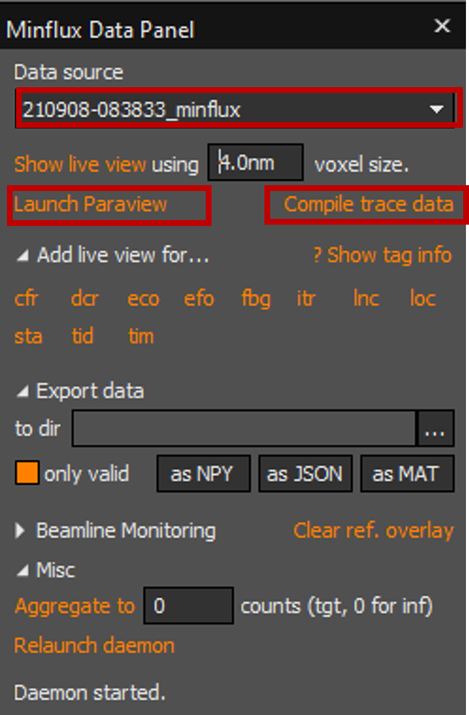
2 **Minflux Data panel** → select data set on **Data source** panel → **Compile trace data** (Trace data compiled on the bottom of Minflux Data panel) **→** then **Launch Paraview [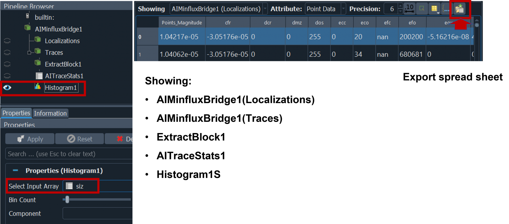](https://www-app.igb.illinois.edu/core-docs/uploads/images/gallery/2022-08/tracking.png)**
3 **ParaView**:
3.1 Localizations: show the dots where molecules were localized:
- loc: localization coordinate; in raw data: determined position of the respective localization in x, y and z
- cfr: center frequency ratio; emission frequency measured at the center pattern position (= efc) divided by emission frequency measured at pattern positions on the circle (= efo)
- dcr: detection channel ratio; emission frequency measured on detector 1 divided by emission frequencies measured on detector 1 + detector 2
- fbg: fluorescence background; determined background level (as count frequency) in the sample
- efo: effective frequency at offset tcp position; emission frequency measured at the pattern positions on the circle (= ”offset”; not in the center position)
- tid: trace ID/identifier
- tim: time; timepoint of localization acquisition in respect to start of the measurement (in seconds)
- itr: iteration
3.2 ExtracBlock1”: the connection between localizations
- Hover Cells on (green triangle): if you click one of the traces this will show you ( block, trace, ID, type, spd, dst) [](https://www-app.igb.illinois.edu/core-docs/uploads/images/gallery/2022-08/tracking-hover-cells-on.png)
4 Traces →**Histogram** → select input Array **(dst, dur, gri, len, mst, siz, tid, tim)**
- Dst: distance from the start point to the end point (it does not follow all the traces) [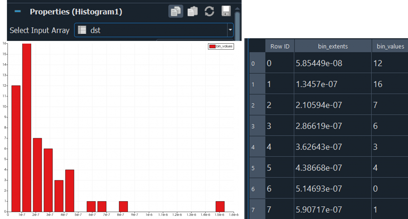](https://www-app.igb.illinois.edu/core-docs/uploads/images/gallery/2022-08/tracking3-dst.png)
- Dur: duration is the total time of the track in second [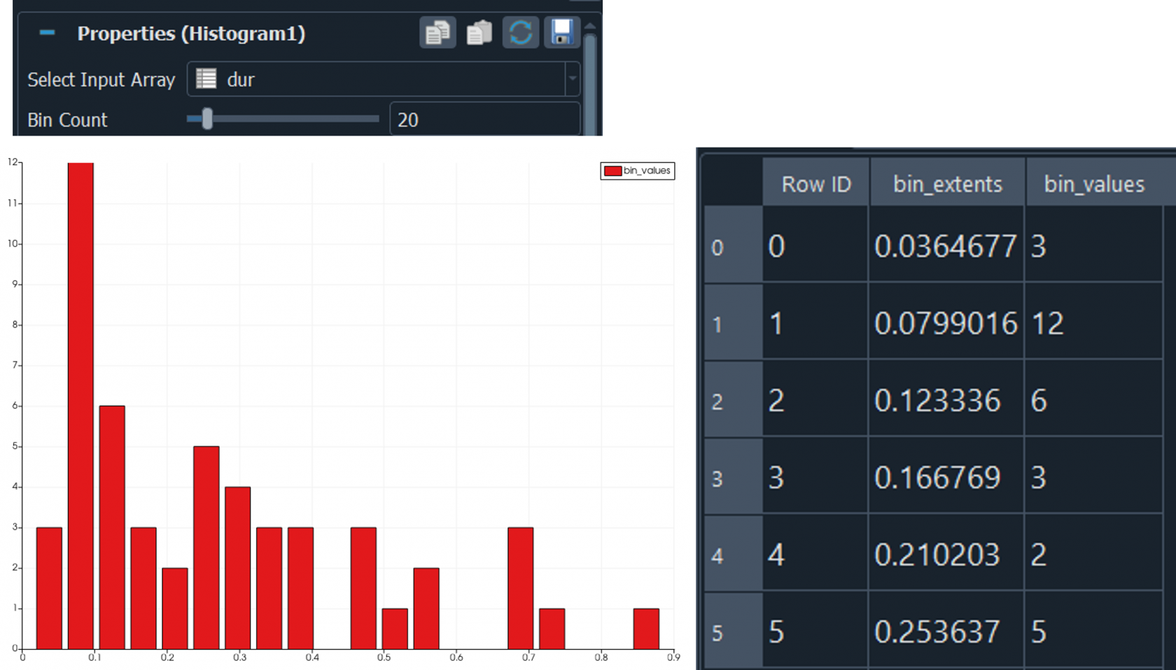](https://www-app.igb.illinois.edu/core-docs/uploads/images/gallery/2022-08/tracking4-dur.png)
- Gri: Grid is scanning point in iteration 0 (this not necessary for histogram)
- Len is the length of completed trace (this is different from dst) [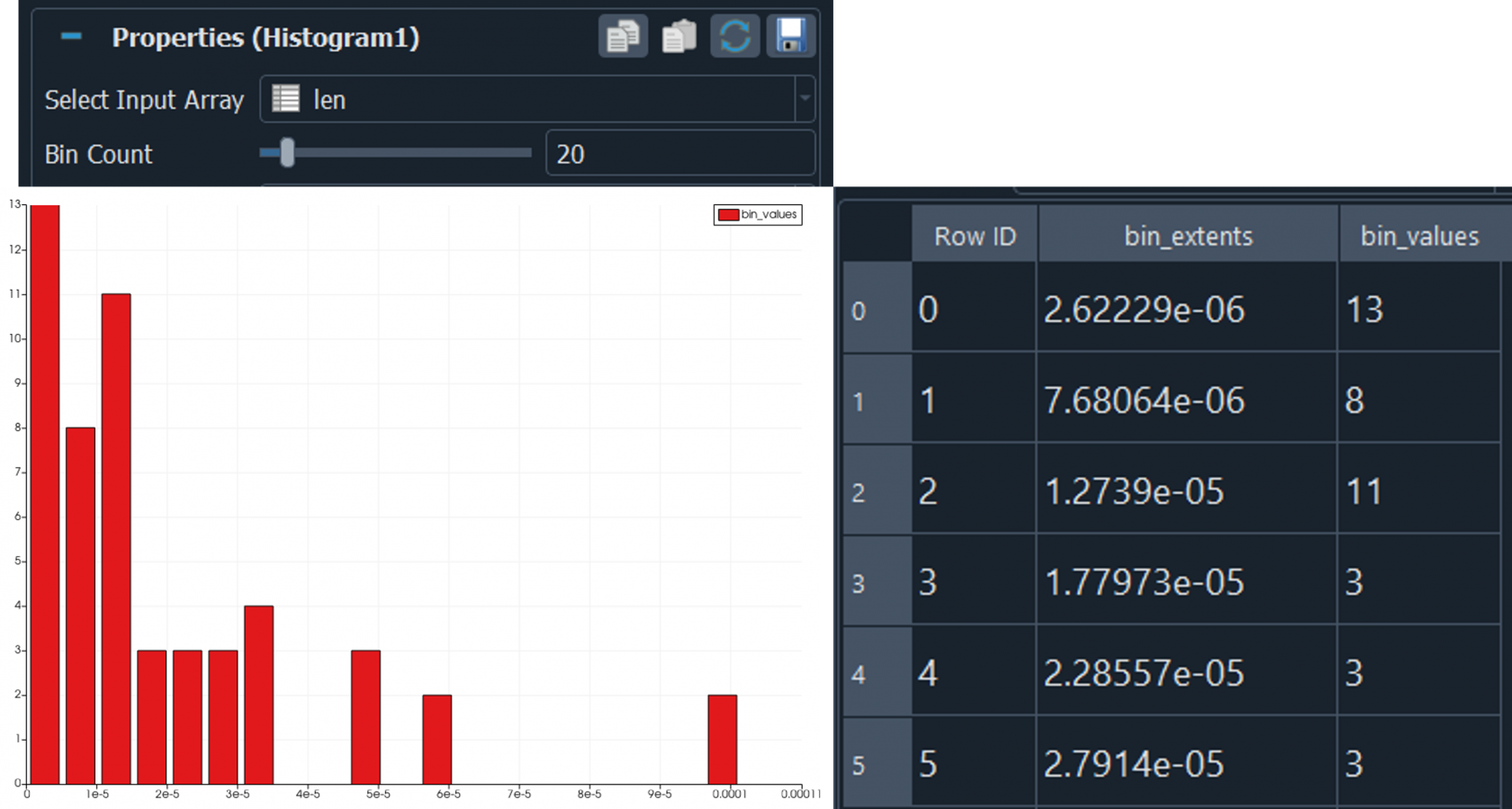](https://www-app.igb.illinois.edu/core-docs/uploads/images/gallery/2022-08/tracking5-len.png)
- mst???? [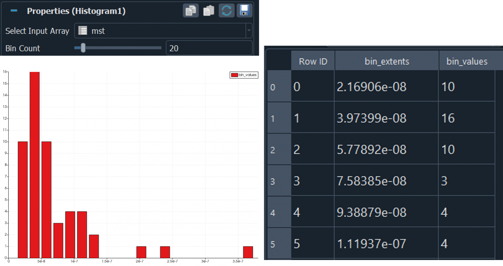](https://www-app.igb.illinois.edu/core-docs/uploads/images/gallery/2022-08/tracking6-mst.png)
- Size is the number of localizations in the trace [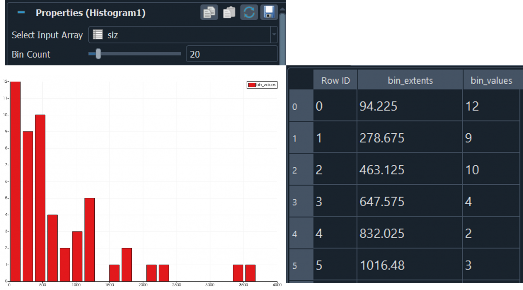](https://www-app.igb.illinois.edu/core-docs/uploads/images/gallery/2022-08/tracking6-siz.png)
5 Traces →**ExtraBlock1**
- Loc: Location of each track, you can color coding based on X, Y or Z
- Tid: random color coding of the traces, by using the traces ID, this similar with Imspector [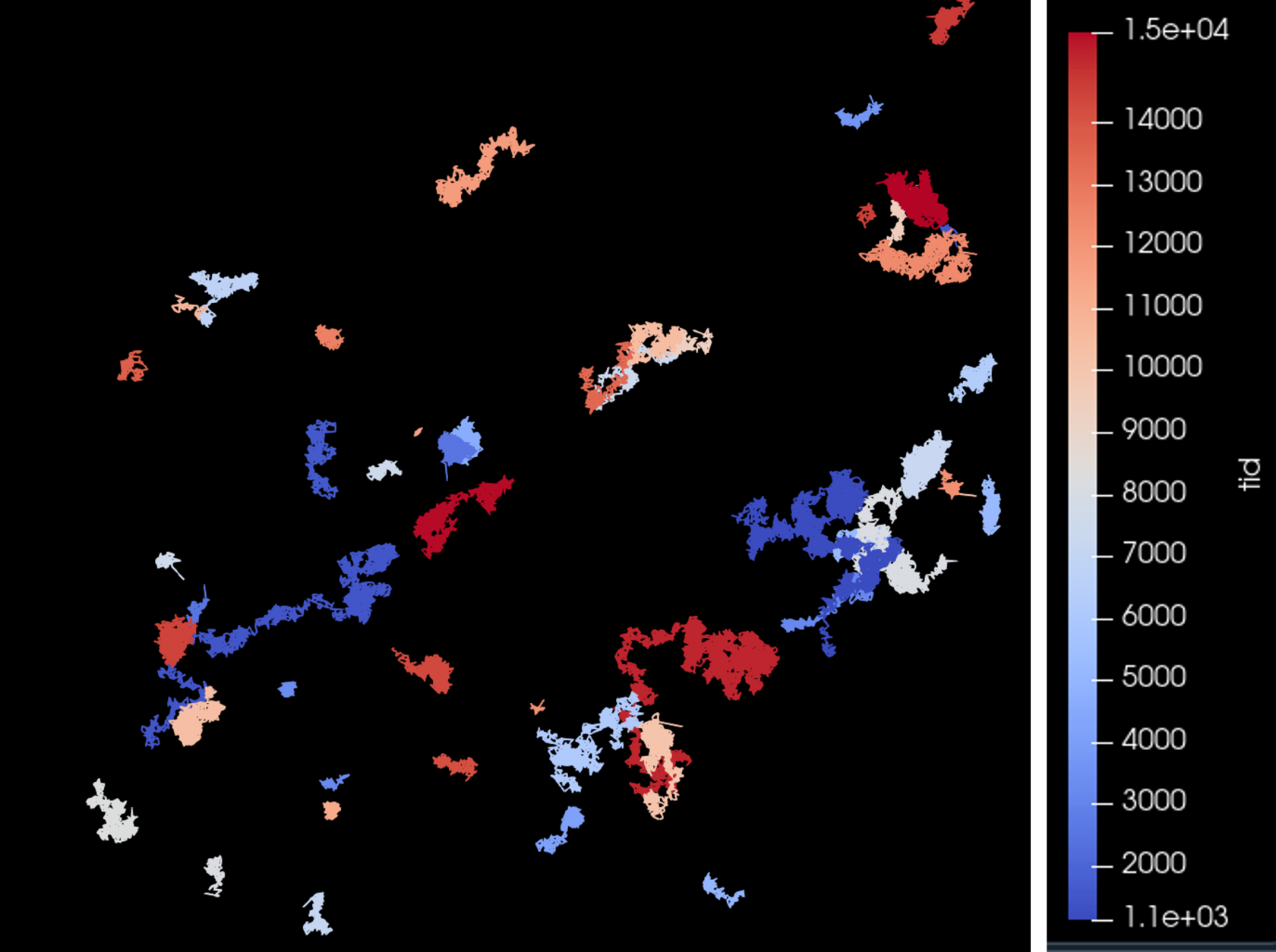](https://www-app.igb.illinois.edu/core-docs/uploads/images/gallery/2022-08/tracking9-tid.png)
- Tim: each localization on the track is color coded regarding the time start of the trace to the end of the trace, (blue to red color coding means blue is the start of the trace and red is the end of the trace). Note: the first localization to the second seem longer than other track [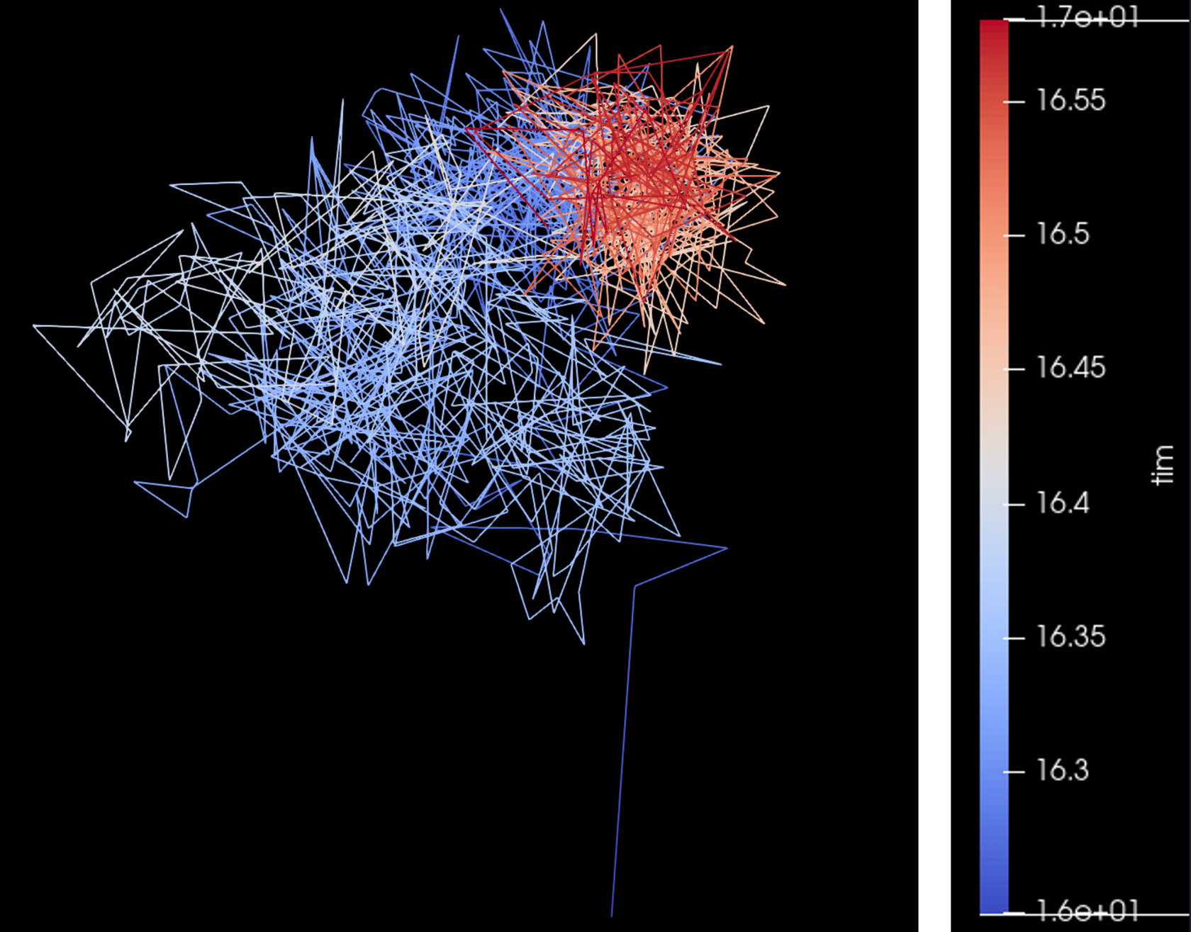](https://www-app.igb.illinois.edu/core-docs/uploads/images/gallery/2022-08/tracking9-tim.png)
- Dst: distance from the start to the end point. Below by using Linear-Green color map show that dark green is the shortest and the white is the longest distance from start localization to the end point/localization. [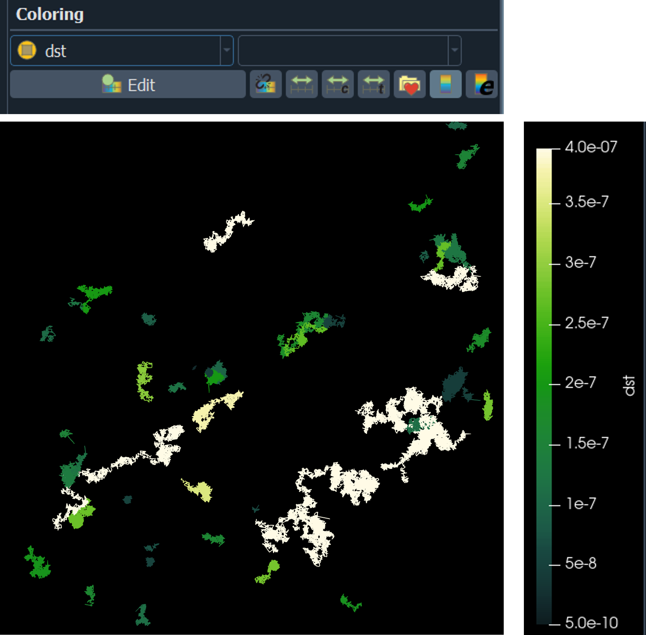](https://www-app.igb.illinois.edu/core-docs/uploads/images/gallery/2022-08/tracking8-dst.png)
- Dst: length between two localizations, the figure we choose one trace dark green is the shortest distance and the white is the longest distance. [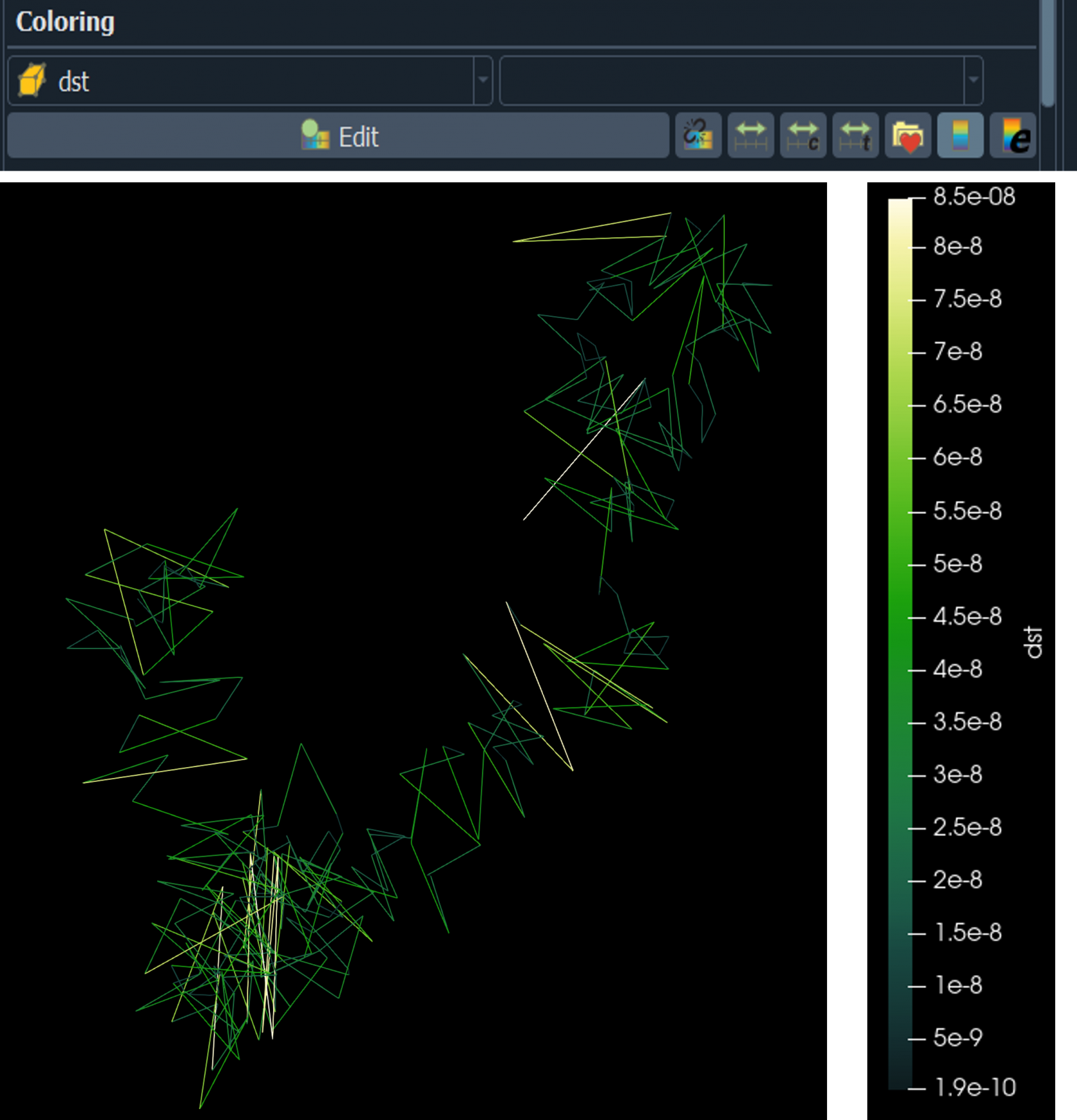](https://www-app.igb.illinois.edu/core-docs/uploads/images/gallery/2022-08/tracking7-dst.png)
- Spd: distance between 2 localizations divided by time [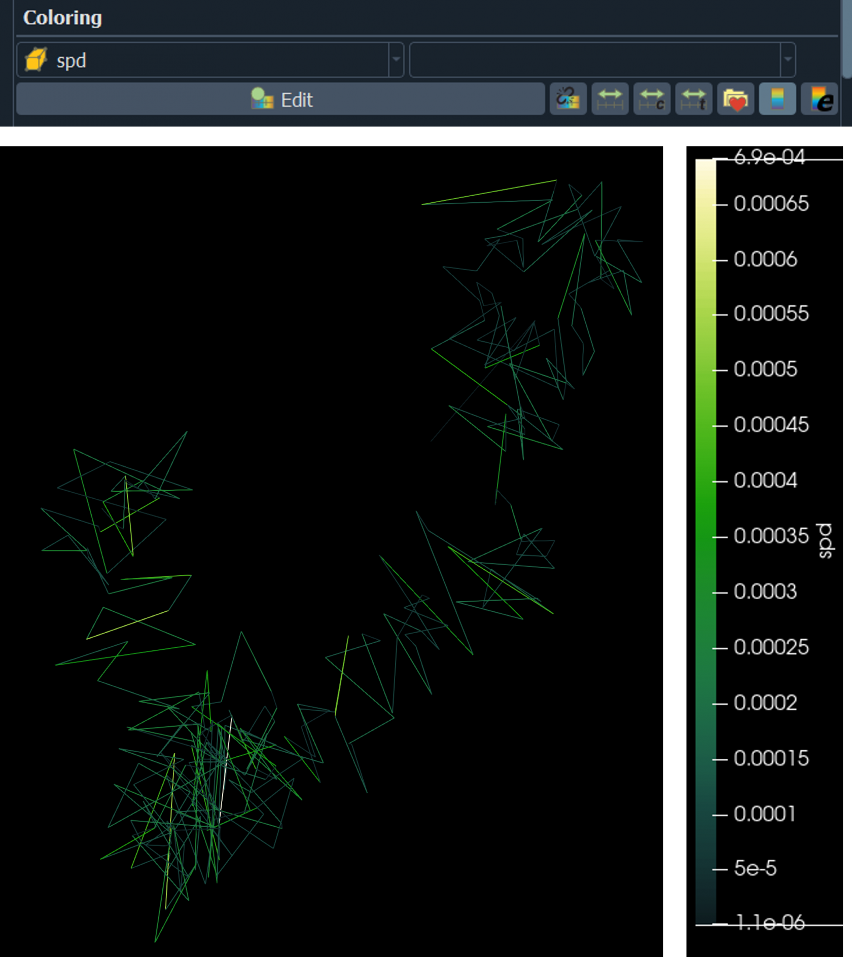](https://www-app.igb.illinois.edu/core-docs/uploads/images/gallery/2022-08/tracking8-spd.png)