# Basic Optics

Initial Training for Optical Microscope Users

# Data Storage

### Store data on the data drive on the local machine:

##### D\\Data may be deleted at anytime. Do not leave your data here! 

##### The core staff will clean the computer drives occasionally. This means that your profile, desktop and data from the data drive will all be removed. We will also remove other files that look like they are not needed.

### Core-Server:

##### The core-server was set up by the IGB Computer Network and Research Group (CNRG) as a place for core users to store their data long term and move it back to your office. You do not need to bring thumb drives or other devices that could bring a computer virus into the core when you come to collect data. Move your data off of the local machine onto the core server at the end of each imaging session. Your PI will have a folder on the core-server and you can make a sub folder for your work. you will have access to all of the sub folders in your PI's folder but not other PI's folders. All of the data in your PI's folder was paid for by your PI and belongs to him/her.

##### Your PI will be charged $8.75/terabyte every month Email [help@igb.illinois.edu](mailto:help@igb.illinois) [for information on charges and tape backup for long term storage. ](mailto:help@igb.illinois)

### Long Term Storage

##### CNRG provides tape backup for long term storage for $200/ terabyte

# Fluorescence Imaging

## Why Fluorescence:

We can label what we want to see

[![image-1636117579202.jpg](https://www-app.igb.illinois.edu/core-docs/uploads/images/gallery/2021-11/scaled-1680-/image-1636117579202.jpg)](https://www-app.igb.illinois.edu/core-docs/uploads/images/gallery/2021-11/image-1636117579202.jpg)

## Excitation and Emission

Dapi

[![image-1636116484648.png](https://www-app.igb.illinois.edu/core-docs/uploads/images/gallery/2021-11/scaled-1680-/image-1636116484648.png)](https://www-app.igb.illinois.edu/core-docs/uploads/images/gallery/2021-11/image-1636116484648.png)

[![image-1636117001582.jpg](https://www-app.igb.illinois.edu/core-docs/uploads/images/gallery/2021-11/scaled-1680-/image-1636117001582.jpg)](https://www-app.igb.illinois.edu/core-docs/uploads/images/gallery/2021-11/image-1636117001582.jpg)

[![image-1636117827645.jpg](https://www-app.igb.illinois.edu/core-docs/uploads/images/gallery/2021-11/scaled-1680-/image-1636117827645.jpg)](https://www-app.igb.illinois.edu/core-docs/uploads/images/gallery/2021-11/image-1636117827645.jpg)

[![image-1636117230797.jpg](https://www-app.igb.illinois.edu/core-docs/uploads/images/gallery/2021-11/scaled-1680-/image-1636117230797.jpg)](https://www-app.igb.illinois.edu/core-docs/uploads/images/gallery/2021-11/image-1636117230797.jpg)

Widefield vs Confocal

[![image-1663333708653.png](https://www-app.igb.illinois.edu/core-docs/uploads/images/gallery/2022-09/scaled-1680-/image-1663333708653.png)](https://www-app.igb.illinois.edu/core-docs/uploads/images/gallery/2022-09/image-1663333708653.png)

[https://www.journals.uchicago.edu/doi/full/10.1086/689588](https://www.journals.uchicago.edu/doi/full/10.1086/689588)

# IGB Core Instrument LSM 880

[![image-1636119638410.png](https://www-app.igb.illinois.edu/core-docs/uploads/images/gallery/2021-11/scaled-1680-/image-1636119638410.png)](https://www-app.igb.illinois.edu/core-docs/uploads/images/gallery/2021-11/image-1636119638410.png)

# IGB Core Instrument LSM 900

[![LSM 900 lightpath.jpg](https://www-app.igb.illinois.edu/core-docs/uploads/images/gallery/2022-12/scaled-1680-/lsm-900-lightpath.jpg)](https://www-app.igb.illinois.edu/core-docs/uploads/images/gallery/2022-12/lsm-900-lightpath.jpg)

405nm, 488nm, 561nm, 640nm excitation.

Zen Blue

file:///C:/Users/gfried/Downloads/EN\_poster\_Beampath-LSM-900\_A1.pdf

# IGB Core Instrument V16


# IGB Core Instruments Axiovert 200M

### Axiovert 200M

[![image-1633538468465.png](https://www-app.igb.illinois.edu/core-docs/uploads/images/gallery/2021-10/scaled-1680-/image-1633538468465.png)](https://www-app.igb.illinois.edu/core-docs/uploads/images/gallery/2021-10/image-1633538468465.png)

#### Cameras

cMOS

# IGB Core Instruments LSM 700

### LSM 700

[![image-1629916880351.png](https://www-app.igb.illinois.edu/core-docs/uploads/images/gallery/2021-08/scaled-1680-/image-1629916880351.png)](https://www-app.igb.illinois.edu/core-docs/uploads/images/gallery/2021-08/image-1629916880351.png)

http://zeiss-campus.magnet.fsu.edu/tutorials/spectralimaging/lsm700/indexflash.html

# IGB Core Instruments Zeiss LSM 710

### Light Path

[![image-1629917181145.png](https://www-app.igb.illinois.edu/core-docs/uploads/images/gallery/2021-08/scaled-1680-/image-1629917181145.png)](https://www-app.igb.illinois.edu/core-docs/uploads/images/gallery/2021-08/image-1629917181145.png)

[https://www.gu.se/en/core-facilities/lsm-710-nlo](https://www.gu.se/en/core-facilities/lsm-710-nlo)

[![image-1633552875050.png](https://www-app.igb.illinois.edu/core-docs/uploads/images/gallery/2021-10/scaled-1680-/image-1633552875050.png)](https://www-app.igb.illinois.edu/core-docs/uploads/images/gallery/2021-10/image-1633552875050.png)

[![image-1633553641518.png](https://www-app.igb.illinois.edu/core-docs/uploads/images/gallery/2021-10/scaled-1680-/image-1633553641518.png)](https://www-app.igb.illinois.edu/core-docs/uploads/images/gallery/2021-10/image-1633553641518.png)

Seven visible excitation lines: 405nm, 458nm, 488nm, 514nm, 561nm, 594nm, 633nm.

Tisaphire laser 700nm to 980nm

<p class="callout info">Spectral Unmixing [http://zeiss-campus.magnet.fsu.edu/articles/spectralimaging/introduction.html](http://zeiss-campus.magnet.fsu.edu/articles/spectralimaging/introduction.html)</p>

<p class="callout info">Multiphoton Microscopy [http://zeiss-campus.magnet.fsu.edu/referencelibrary/multiphoton.html ](http://zeiss-campus.magnet.fsu.edu/articles/spectralimaging/introduction.html)</p>

<p class="callout info">Fluorescence Lifetime Imaging Microscopy (FLIM) http://www.iss.com/microscopy/components/FastFLIM.html</p>

# Objectives


# Optics

## Properties of light

### Wave particle duality:

Light is a wave

![](https://latex.codecogs.com/svg.image?E=h%5Cnu&space;were&space;E&space;is&space;energy,&space;h&space;is&space;planks&space;constant&space;and&space;%5Cnu&space;is&space;frequancy "E=h\nu were E is energy, h is planks constant and \nu is frequancy")

[![image-1630006591207.png](https://www-app.igb.illinois.edu/core-docs/uploads/images/gallery/2021-08/scaled-1680-/image-1630006591207.png)
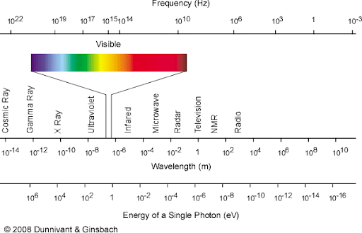
](https://www-app.igb.illinois.edu/core-docs/uploads/images/gallery/2021-08/image-1630006591207.png)

### Absorption and Emission

Beer's law

Refraction

## Ray tracing

## Resolution

### **Resolution:** The ability to separate two objects

[![image-1633036148165.jpg](https://www-app.igb.illinois.edu/core-docs/uploads/images/gallery/2021-09/scaled-1680-/image-1633036148165.jpg)
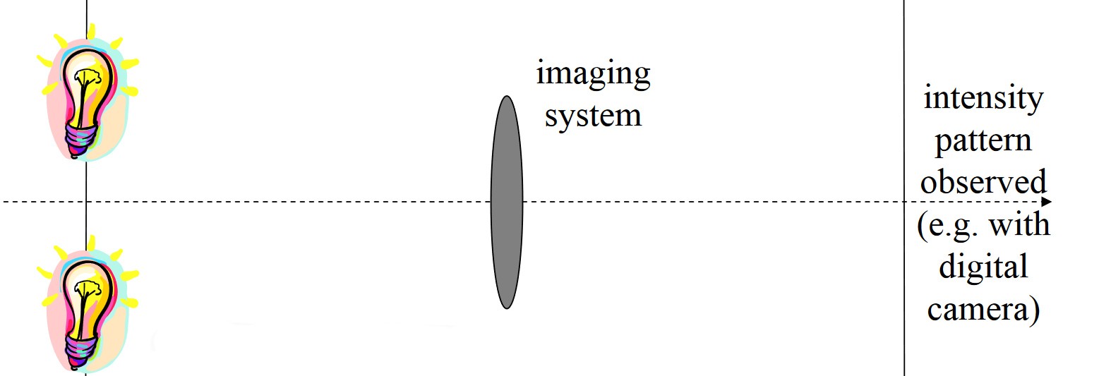
](https://www-app.igb.illinois.edu/core-docs/uploads/images/gallery/2021-09/image-1633036148165.jpg)

### **A definition of Numerical Aperture**

[![image-1633036910068.jpg](https://www-app.igb.illinois.edu/core-docs/uploads/images/gallery/2021-09/scaled-1680-/image-1633036910068.jpg)
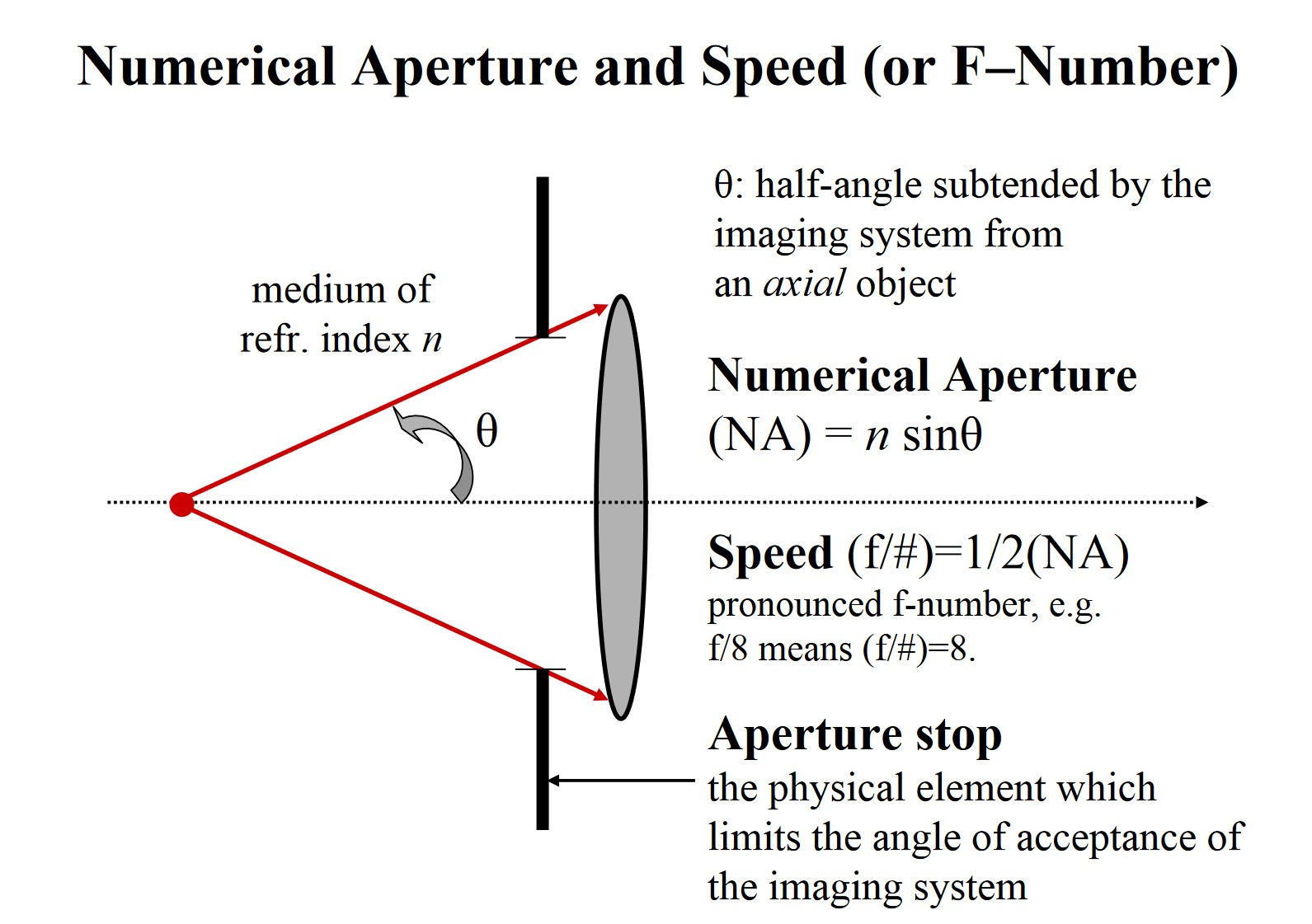
](https://www-app.igb.illinois.edu/core-docs/uploads/images/gallery/2021-09/image-1633036910068.jpg)

#### Fourier transform:

Transform from real space to frequency space

[![image-1636115576367.jpg](https://www-app.igb.illinois.edu/core-docs/uploads/images/gallery/2021-11/scaled-1680-/image-1636115576367.jpg)
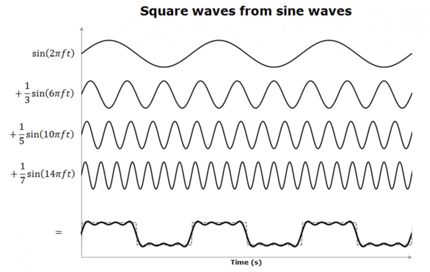
](https://www-app.igb.illinois.edu/core-docs/uploads/images/gallery/2021-11/image-1636115576367.jpg)

Now we look at a real square wave and frequency space

[![image-1636115856897.jpg](https://www-app.igb.illinois.edu/core-docs/uploads/images/gallery/2021-11/scaled-1680-/image-1636115856897.jpg)
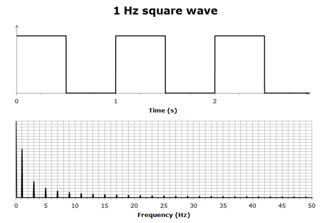
](https://www-app.igb.illinois.edu/core-docs/uploads/images/gallery/2021-11/image-1636115856897.jpg)

### **Look at a simple optical system:**

[![image-1633036975307.jpg](https://www-app.igb.illinois.edu/core-docs/uploads/images/gallery/2021-09/scaled-1680-/image-1633036975307.jpg)
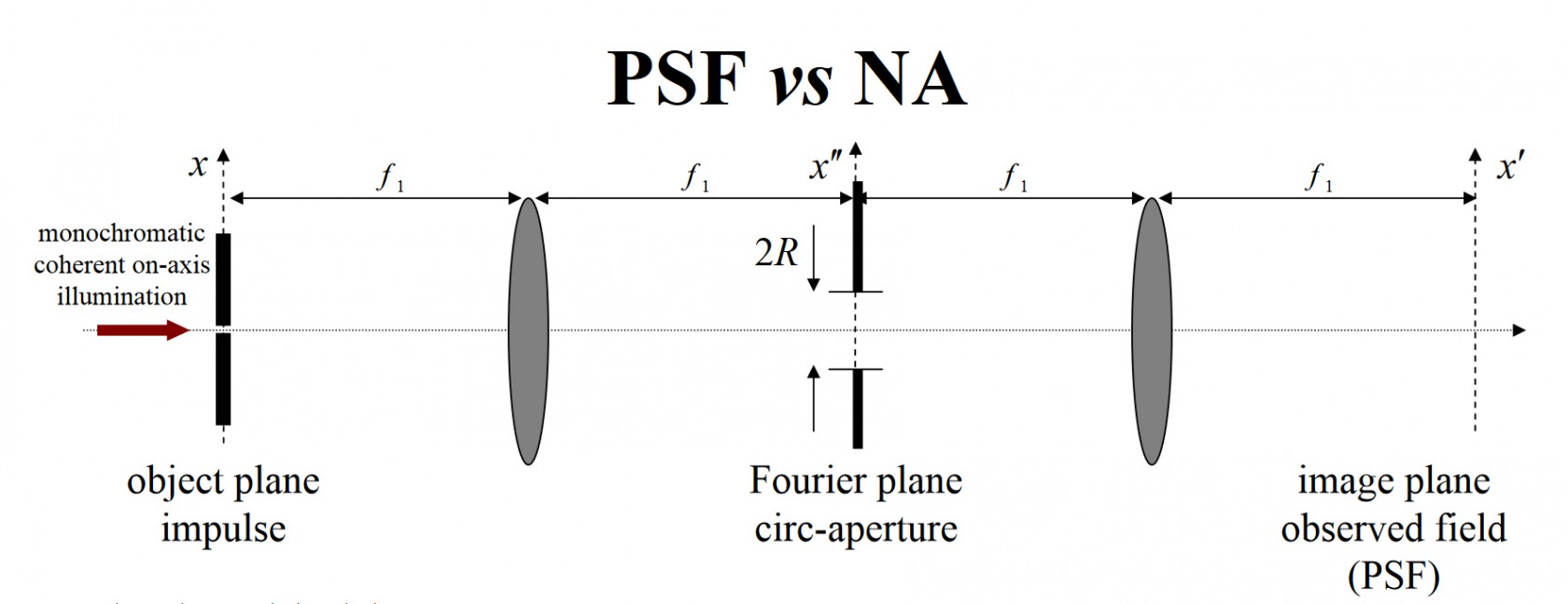
](https://www-app.igb.illinois.edu/core-docs/uploads/images/gallery/2021-09/image-1633036975307.jpg)

#### Mathematical prediction of the Point Spread Function (PSF)

on the left we have the mathematical point source know as a delta function.

[![image-1633098662004.jpg](https://www-app.igb.illinois.edu/core-docs/uploads/images/gallery/2021-10/scaled-1680-/image-1633098662004.jpg)
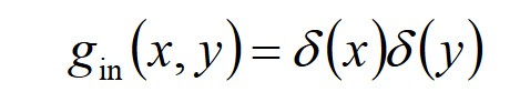
](https://www-app.igb.illinois.edu/core-docs/uploads/images/gallery/2021-10/image-1633098662004.jpg)

were

[![image-1633098725511.jpg](https://www-app.igb.illinois.edu/core-docs/uploads/images/gallery/2021-10/scaled-1680-/image-1633098725511.jpg)
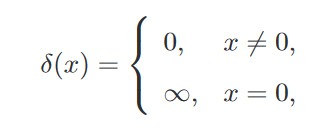
](https://www-app.igb.illinois.edu/core-docs/uploads/images/gallery/2021-10/image-1633098725511.jpg)

the intensity at the Fourier plain can be found by taking the Fourier transform of this function.

[![image-1633098872812.jpg](https://www-app.igb.illinois.edu/core-docs/uploads/images/gallery/2021-10/scaled-1680-/image-1633098872812.jpg) 
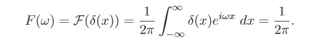
or ](https://www-app.igb.illinois.edu/core-docs/uploads/images/gallery/2021-10/image-1633098872812.jpg)

[![image-1633100310895.jpg](https://www-app.igb.illinois.edu/core-docs/uploads/images/gallery/2021-10/scaled-1680-/image-1633100310895.jpg)
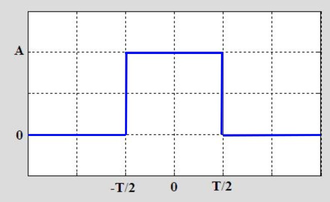
](https://www-app.igb.illinois.edu/core-docs/uploads/images/gallery/2021-10/image-1633100310895.jpg)

this has the same intensity at all points inside the aperture and zero outside. The second lens is now taking a Fourier transform on a box function the width of the aperture.

[![image-1633099073037.jpg](https://www-app.igb.illinois.edu/core-docs/uploads/images/gallery/2021-10/scaled-1680-/image-1633099073037.jpg)
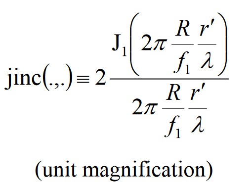
](https://www-app.igb.illinois.edu/core-docs/uploads/images/gallery/2021-10/image-1633099073037.jpg)

or

[![image-1633100364032.jpg](https://www-app.igb.illinois.edu/core-docs/uploads/images/gallery/2021-10/scaled-1680-/image-1633100364032.jpg)
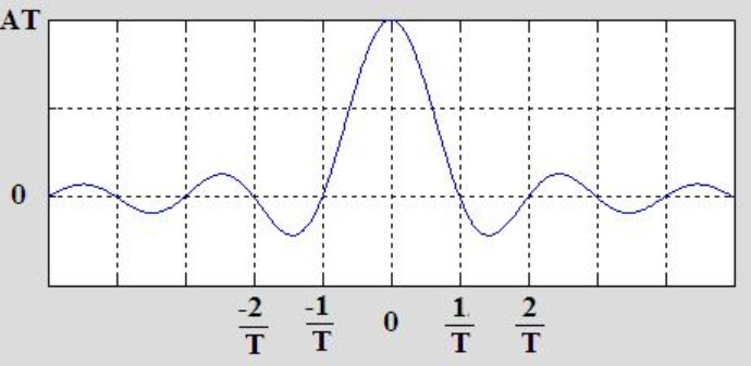
](https://www-app.igb.illinois.edu/core-docs/uploads/images/gallery/2021-10/image-1633100364032.jpg)

Substituting in the definition for NA

[![image-1633101363801.jpg](https://www-app.igb.illinois.edu/core-docs/uploads/images/gallery/2021-10/scaled-1680-/image-1633101363801.jpg)
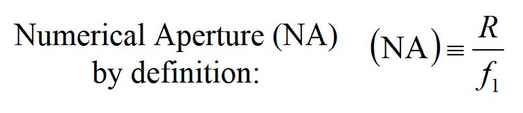
](https://www-app.igb.illinois.edu/core-docs/uploads/images/gallery/2021-10/image-1633101363801.jpg)

[![image-1633101383326.jpg](https://www-app.igb.illinois.edu/core-docs/uploads/images/gallery/2021-10/scaled-1680-/image-1633101383326.jpg)
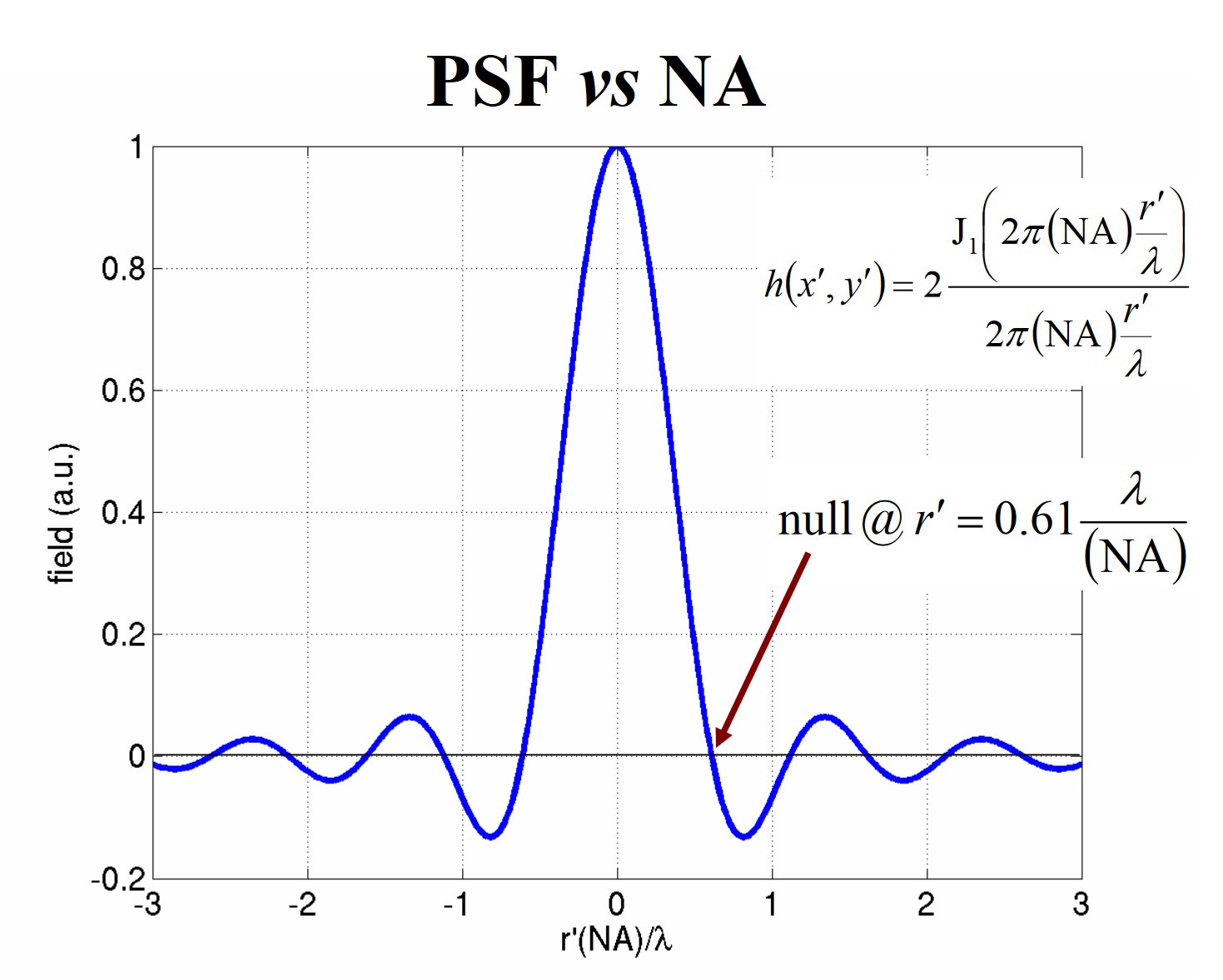
](https://www-app.igb.illinois.edu/core-docs/uploads/images/gallery/2021-10/image-1633101383326.jpg)

[![image-1633102388922.jpg](https://www-app.igb.illinois.edu/core-docs/uploads/images/gallery/2021-10/scaled-1680-/image-1633102388922.jpg)
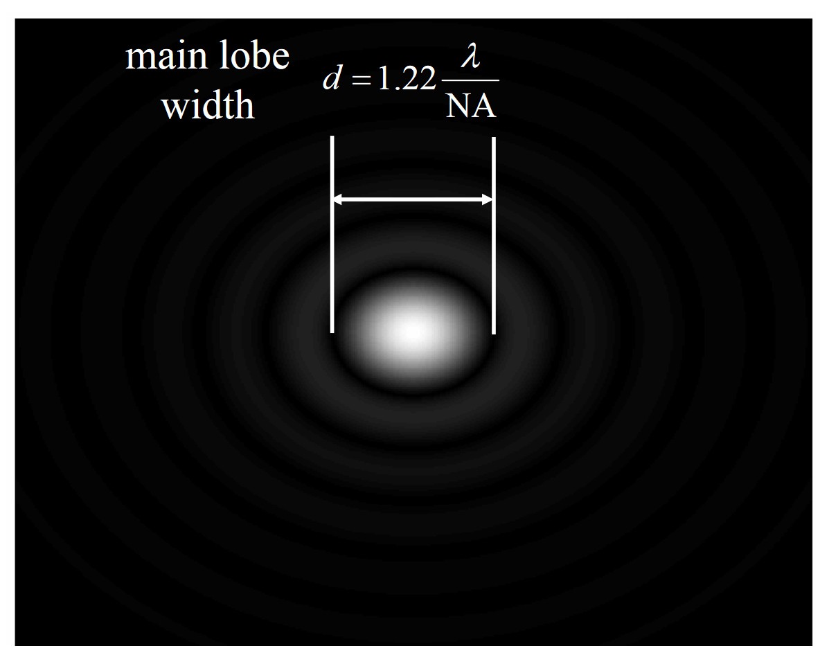
](https://www-app.igb.illinois.edu/core-docs/uploads/images/gallery/2021-10/image-1633102388922.jpg)

[![image-1633102956154.jpg](https://www-app.igb.illinois.edu/core-docs/uploads/images/gallery/2021-10/scaled-1680-/image-1633102956154.jpg)
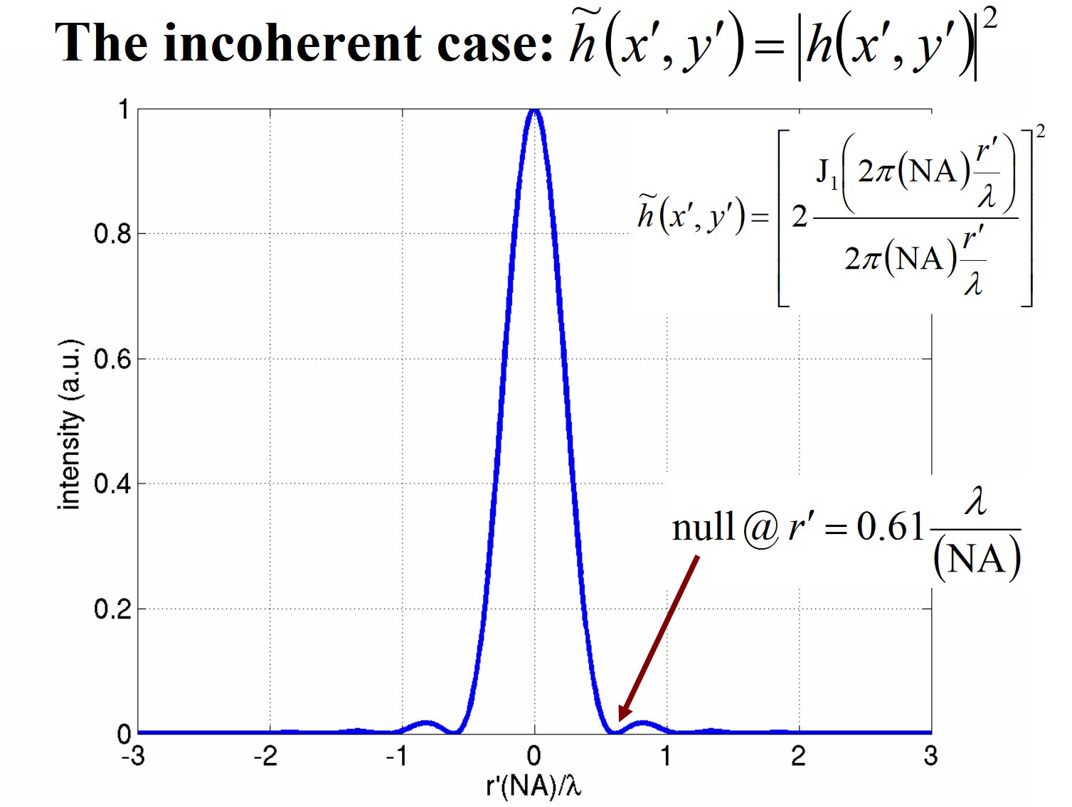
](https://www-app.igb.illinois.edu/core-docs/uploads/images/gallery/2021-10/image-1633102956154.jpg)

### Now we go back to Resolution. How close together we can position two points and still distinguish them

[![image-1633114549481.jpg](https://www-app.igb.illinois.edu/core-docs/uploads/images/gallery/2021-10/scaled-1680-/image-1633114549481.jpg)
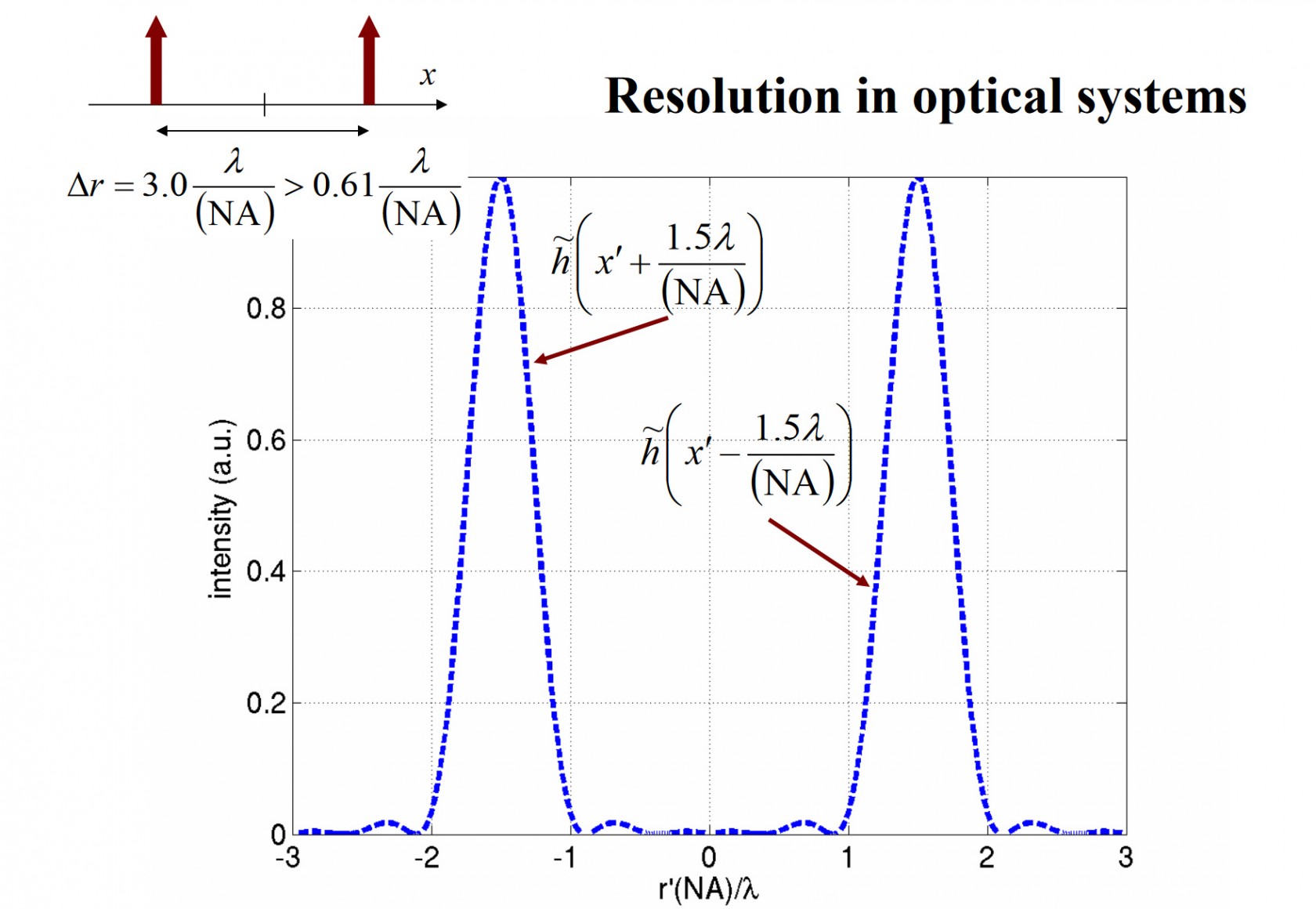
](https://www-app.igb.illinois.edu/core-docs/uploads/images/gallery/2021-10/image-1633114549481.jpg)

[![image-1633114570726.jpg](https://www-app.igb.illinois.edu/core-docs/uploads/images/gallery/2021-10/scaled-1680-/image-1633114570726.jpg)
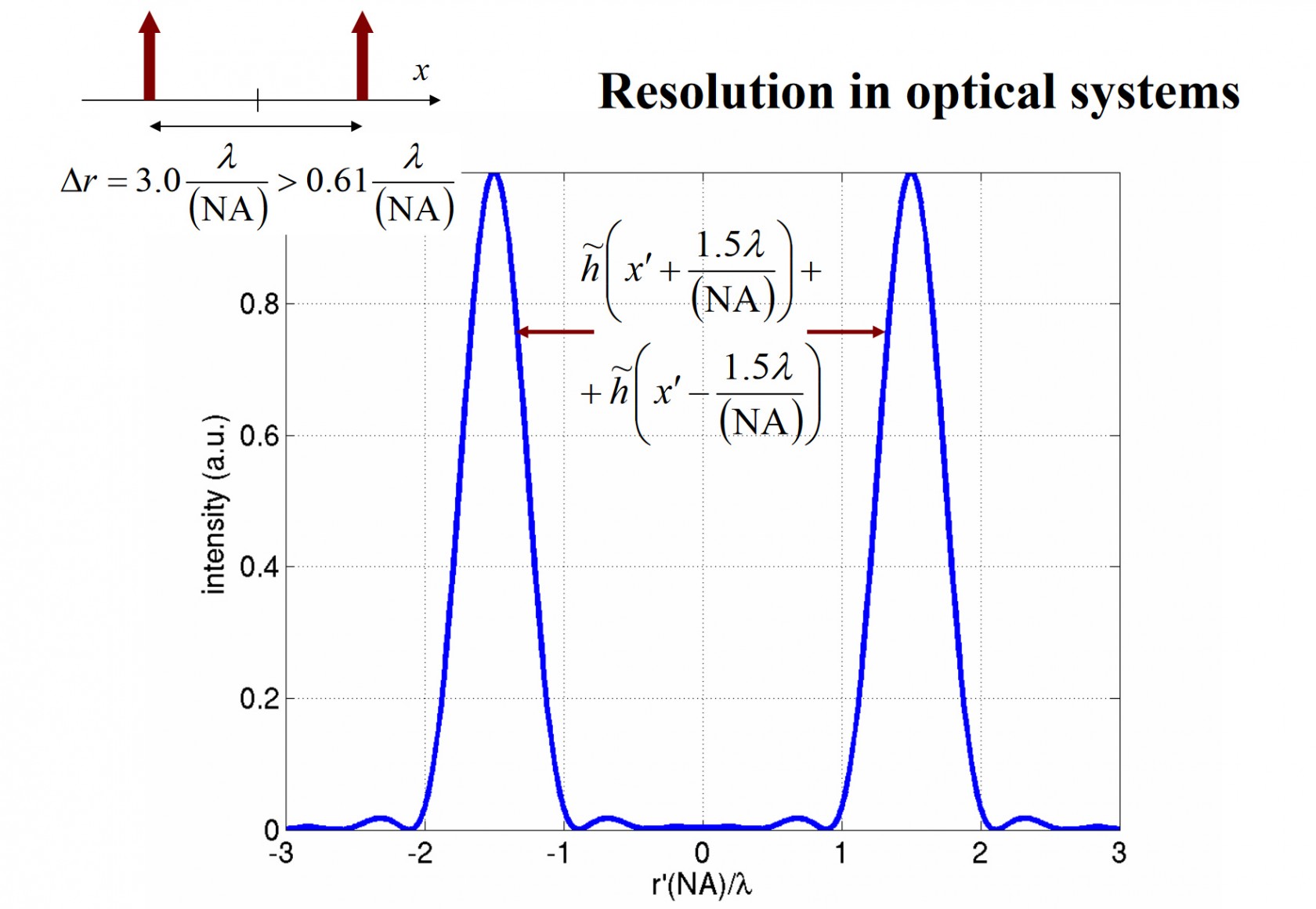
](https://www-app.igb.illinois.edu/core-docs/uploads/images/gallery/2021-10/image-1633114570726.jpg)

[![image-1633114634257.jpg](https://www-app.igb.illinois.edu/core-docs/uploads/images/gallery/2021-10/scaled-1680-/image-1633114634257.jpg)
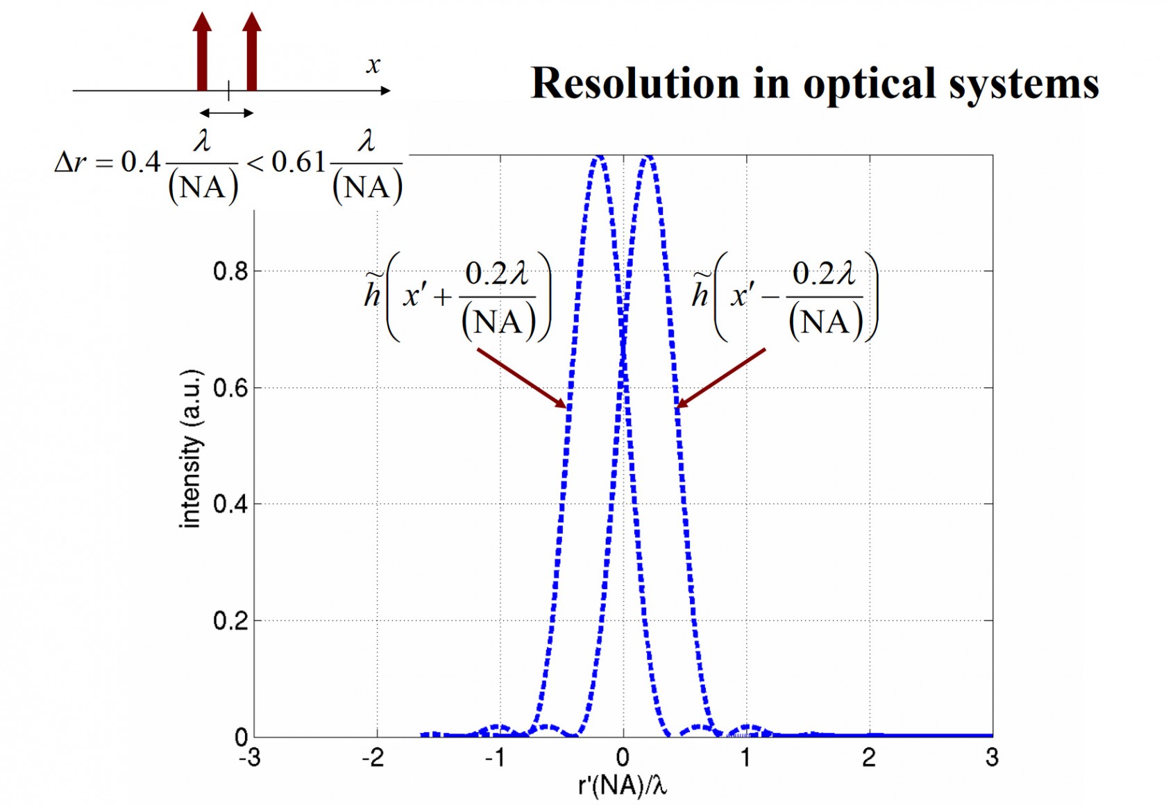
](https://www-app.igb.illinois.edu/core-docs/uploads/images/gallery/2021-10/image-1633114634257.jpg)

[![image-1633114702326.jpg](https://www-app.igb.illinois.edu/core-docs/uploads/images/gallery/2021-10/scaled-1680-/image-1633114702326.jpg)
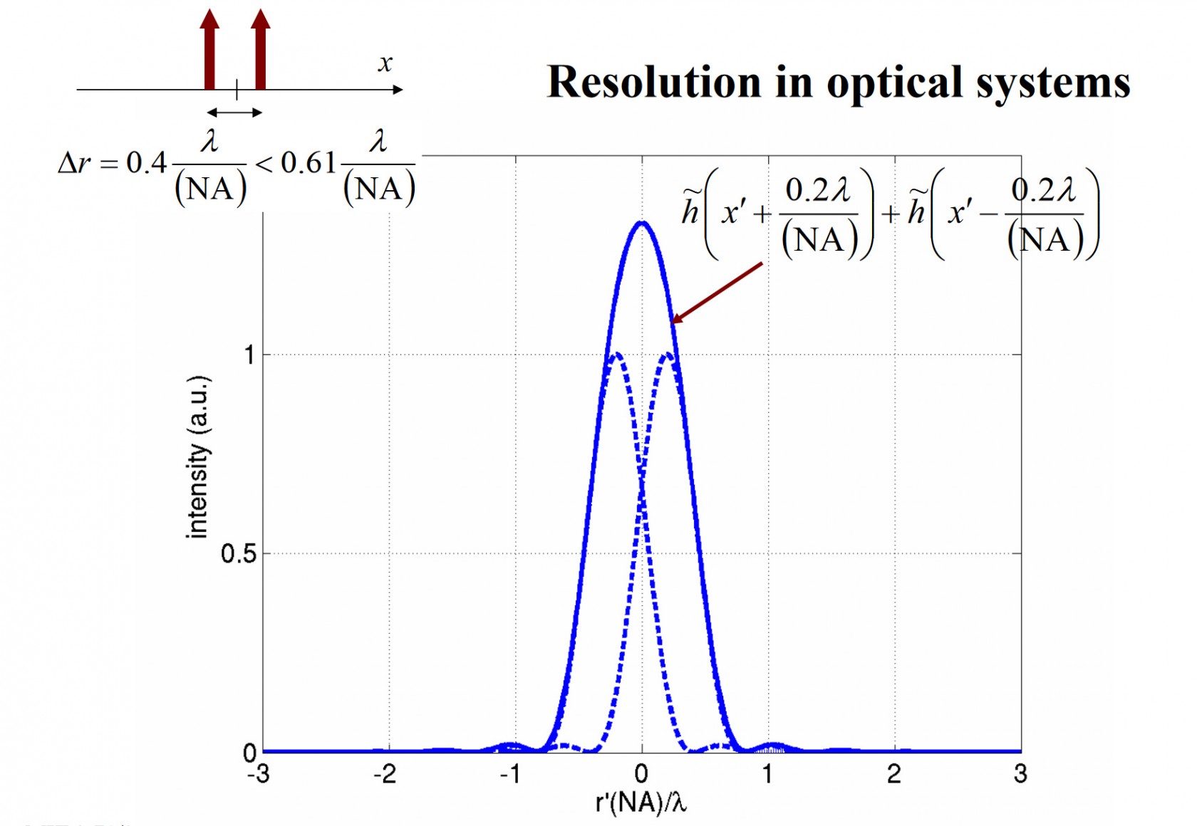
](https://www-app.igb.illinois.edu/core-docs/uploads/images/gallery/2021-10/image-1633114702326.jpg)

[![image-1633114780018.jpg](https://www-app.igb.illinois.edu/core-docs/uploads/images/gallery/2021-10/scaled-1680-/image-1633114780018.jpg)
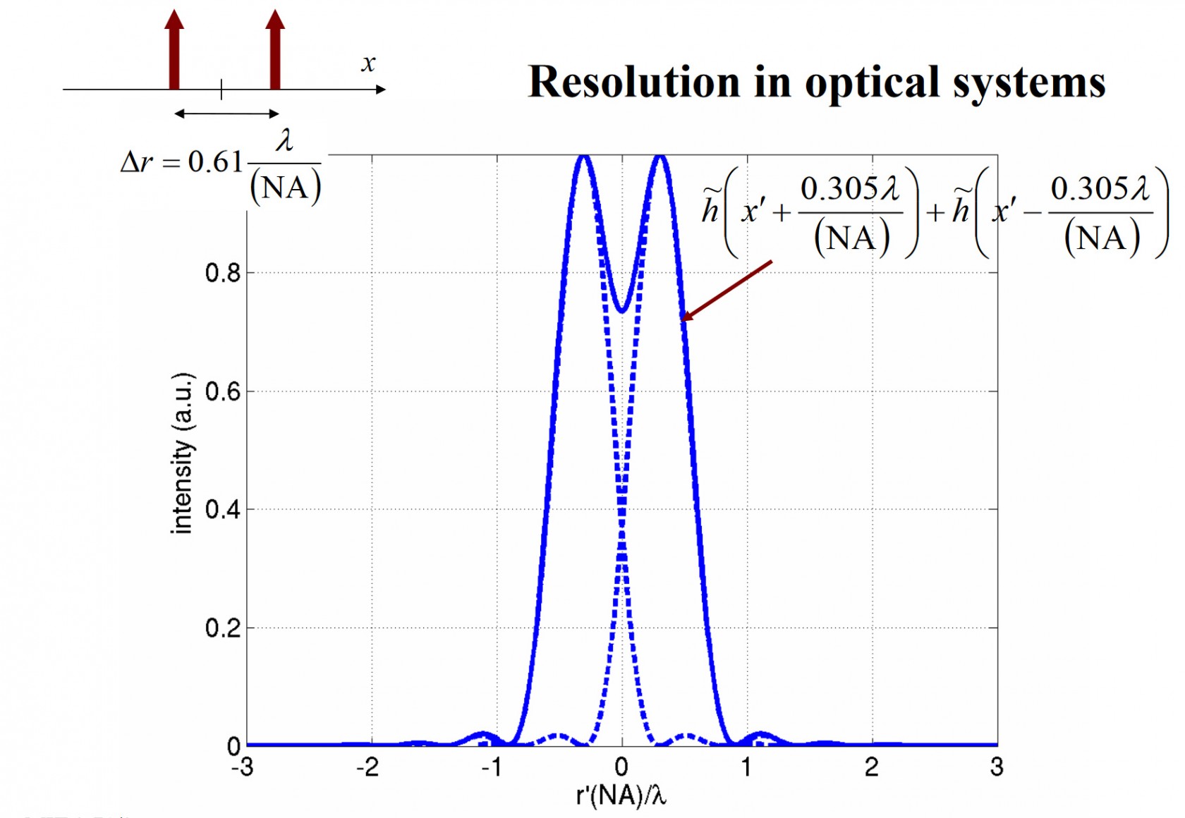
](https://www-app.igb.illinois.edu/core-docs/uploads/images/gallery/2021-10/image-1633114780018.jpg)

[![image-1633114748922.jpg](https://www-app.igb.illinois.edu/core-docs/uploads/images/gallery/2021-10/scaled-1680-/image-1633114748922.jpg)
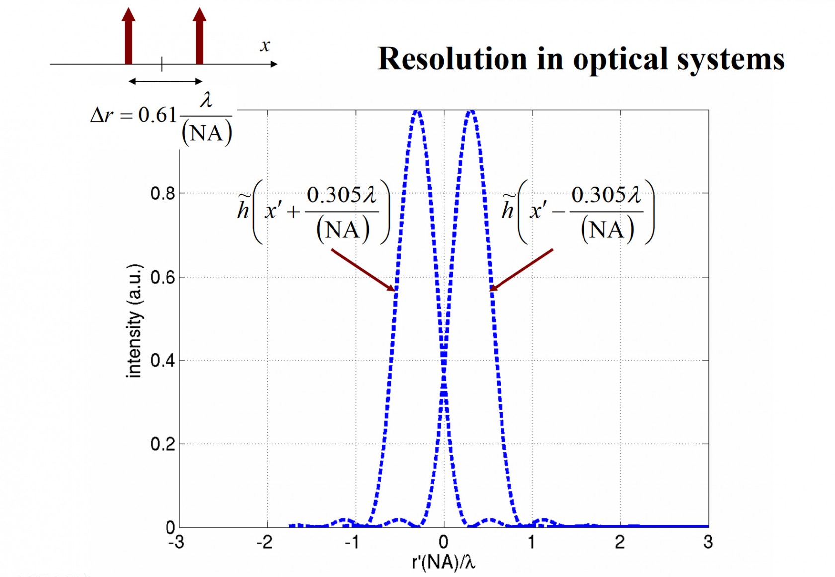
](https://www-app.igb.illinois.edu/core-docs/uploads/images/gallery/2021-10/image-1633114748922.jpg)

[![image-1633115867409.jpg](https://www-app.igb.illinois.edu/core-docs/uploads/images/gallery/2021-10/scaled-1680-/image-1633115867409.jpg)
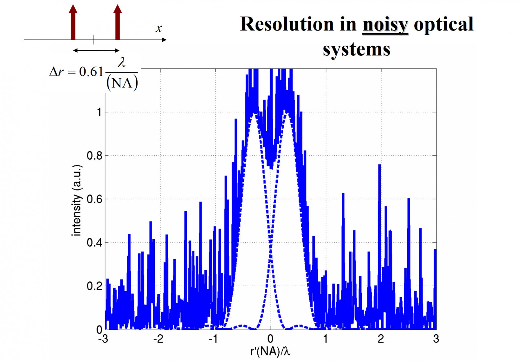
](https://www-app.igb.illinois.edu/core-docs/uploads/images/gallery/2021-10/image-1633115867409.jpg)

[![image-1633115434455.jpg](https://www-app.igb.illinois.edu/core-docs/uploads/images/gallery/2021-10/scaled-1680-/image-1633115434455.jpg)](https://www-app.igb.illinois.edu/core-docs/uploads/images/gallery/2021-10/image-1633115434455.jpg)

[![image-1633697496290.jpg](https://www-app.igb.illinois.edu/core-docs/uploads/images/gallery/2021-10/scaled-1680-/image-1633697496290.jpg)
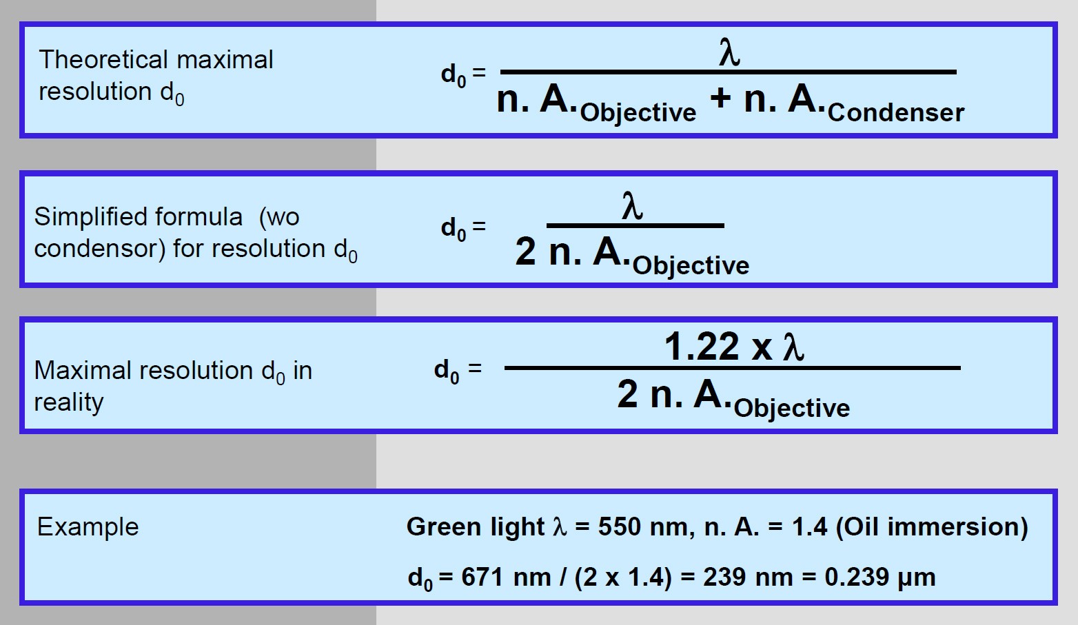
](https://www-app.igb.illinois.edu/core-docs/uploads/images/gallery/2021-10/image-1633697496290.jpg)

More intuitive approach

[![image-1633697667324.jpg](https://www-app.igb.illinois.edu/core-docs/uploads/images/gallery/2021-10/scaled-1680-/image-1633697667324.jpg)
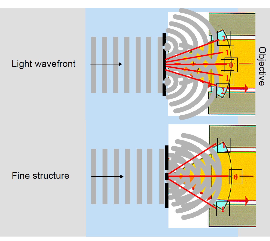
](https://www-app.igb.illinois.edu/core-docs/uploads/images/gallery/2021-10/image-1633697667324.jpg)

Notes from:

[http://web.mit.edu/2.710/Fall06/2.710-wk12-b-sl.pdf](http://web.mit.edu/2.710/Fall06/2.710-wk12-b-sl.pdf)

[https://links.uwaterloo.ca/amath353docs/set11.pdf](https://links.uwaterloo.ca/amath353docs/set11.pdf)

[https://www.thefouriertransform.com/pairs/box.php](https://www.thefouriertransform.com/pairs/box.php)

[http://www.phys.unm.edu/msbahae/Optics%20Lab/Fourier%20Optics.pdf](http://www.phys.unm.edu/msbahae/Optics%20Lab/Fourier%20Optics.pdf)

How to Chose the Optimal Objective Dr. Sebastian Gliem

## Super Resolution Techniques

# Sampling

## How does digital sampling affect resolution

##### Look at imaging these object with a digital camera

##### How close together do pixels need to be?

[![image-1637163325668.jpg](https://www-app.igb.illinois.edu/core-docs/uploads/images/gallery/2021-11/scaled-1680-/image-1637163325668.jpg)
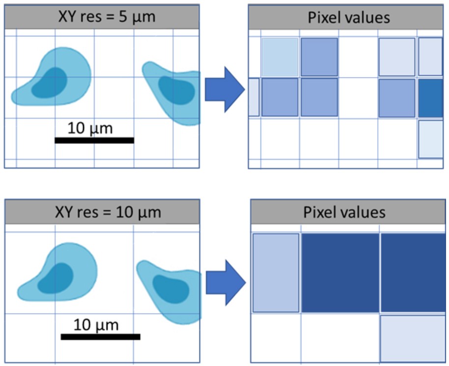
](https://www-app.igb.illinois.edu/core-docs/uploads/images/gallery/2021-11/image-1637163325668.jpg)

##### Sampling over time:

##### How often do you need to image a moving sample

[![image-1637163343425.jpg](https://www-app.igb.illinois.edu/core-docs/uploads/images/gallery/2021-11/scaled-1680-/image-1637163343425.jpg)
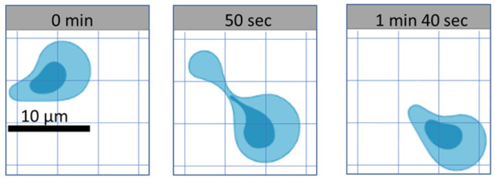
](https://www-app.igb.illinois.edu/core-docs/uploads/images/gallery/2021-11/image-1637163343425.jpg)

### Nyquist theory states that you should sample more than 2 X the frequency that you expect.

#### Over sampling

[![image-1637166398425.jpg](https://www-app.igb.illinois.edu/core-docs/uploads/images/gallery/2021-11/scaled-1680-/image-1637166398425.jpg)
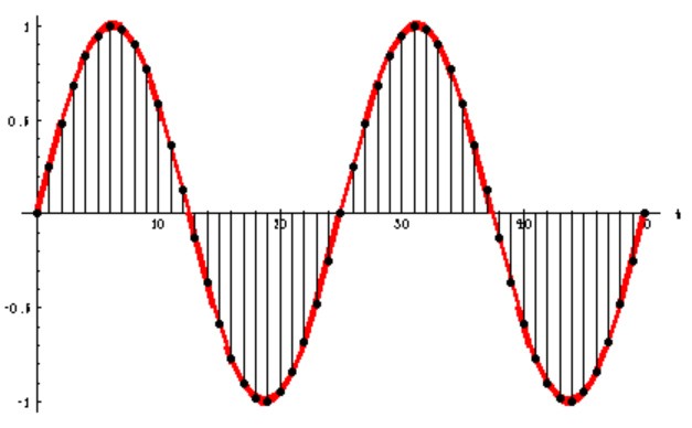
](https://www-app.igb.illinois.edu/core-docs/uploads/images/gallery/2021-11/image-1637166398425.jpg)

#### Nyquist sampling

[![image-1637166436296.jpg](https://www-app.igb.illinois.edu/core-docs/uploads/images/gallery/2021-11/scaled-1680-/image-1637166436296.jpg)
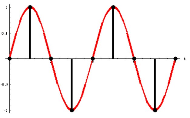
](https://www-app.igb.illinois.edu/core-docs/uploads/images/gallery/2021-11/image-1637166436296.jpg)

#### Under sampling causes aliasing

[![image-1637166449555.jpg](https://www-app.igb.illinois.edu/core-docs/uploads/images/gallery/2021-11/scaled-1680-/image-1637166449555.jpg)
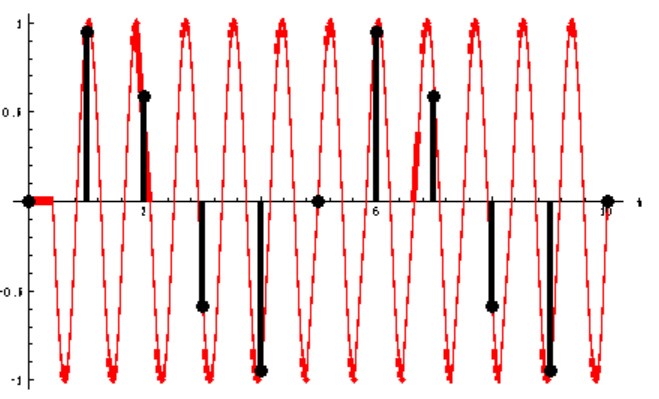
](https://www-app.igb.illinois.edu/core-docs/uploads/images/gallery/2021-11/image-1637166449555.jpg)

### Optical Transfer Function MTF

[![image-1637271420704.jpg](https://www-app.igb.illinois.edu/core-docs/uploads/images/gallery/2021-11/scaled-1680-/image-1637271420704.jpg)
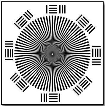
](https://www-app.igb.illinois.edu/core-docs/uploads/images/gallery/2021-11/image-1637271420704.jpg)[ ](https://www-app.igb.illinois.edu/core-docs/uploads/images/gallery/2021-11/image-1637272498227.jpg)[![image-1637272536733.png](https://www-app.igb.illinois.edu/core-docs/uploads/images/gallery/2021-11/scaled-1680-/image-1637272536733.png)
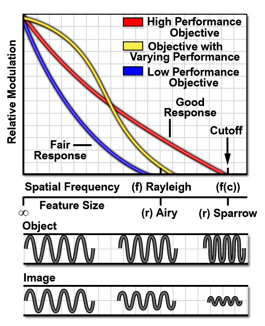
](https://www-app.igb.illinois.edu/core-docs/uploads/images/gallery/2021-11/image-1637272536733.png)

### When objects get close together the contrast decreases.

##### MTF = Image Modulation/Object Modulation

##### MTF = 2(φ - cosφsinφ)/π and 

#####  φ = cos<sup>-1</sup>(λν/2NA)

#####  

##### The Optical Transfer function is the Modulation transfer function times a phase component.

##### OTF = MTF × eiφ(f)

### Camera bit depth

 0 or 1

00 or 01 or 10 or 11

000 or 001 or 010 or 011 or 100 or 101 or 110 or 111

and so on

[ ![image-1637330338226.jpg](https://www-app.igb.illinois.edu/core-docs/uploads/images/gallery/2021-11/scaled-1680-/image-1637330338226.jpg)
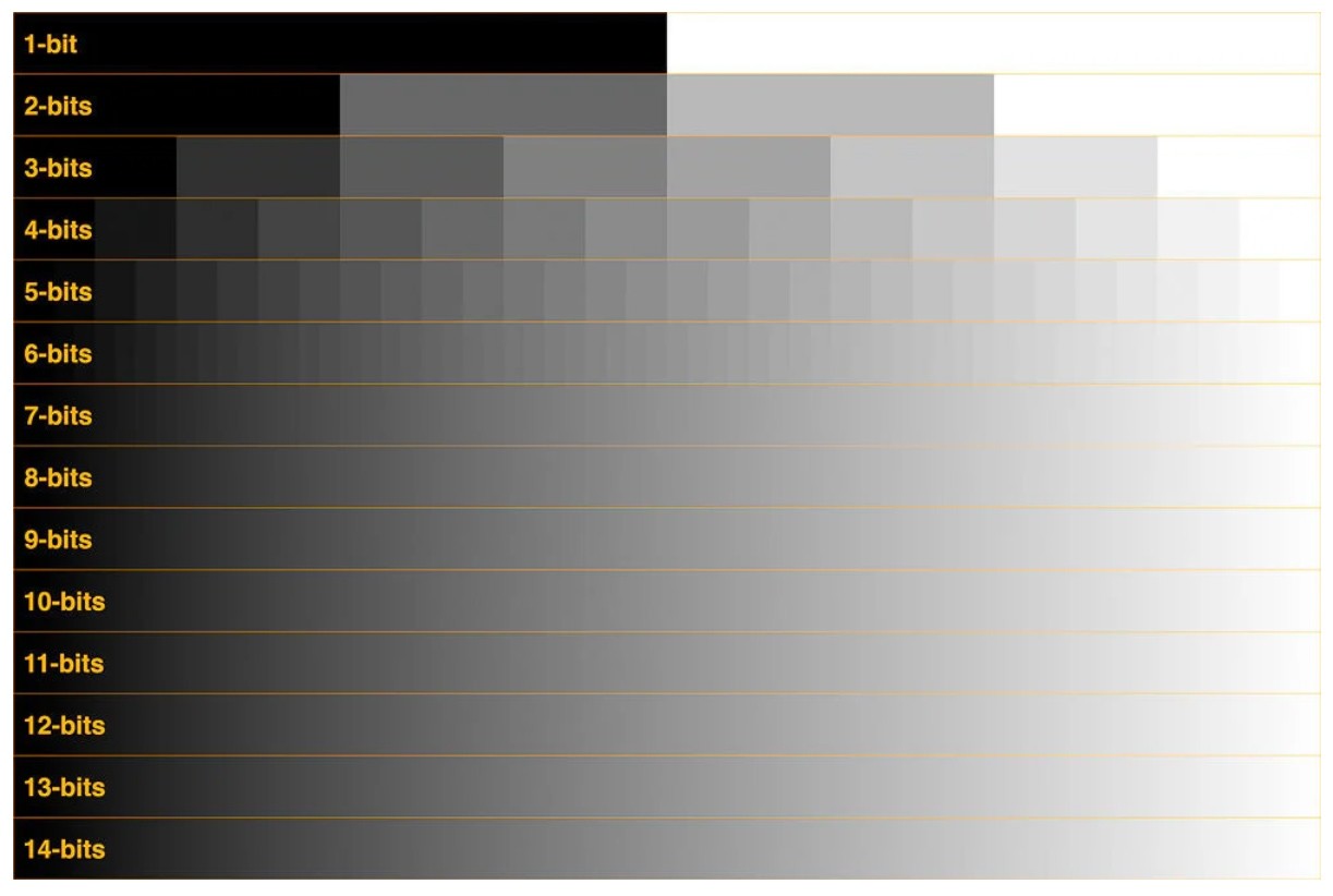
](https://www-app.igb.illinois.edu/core-docs/uploads/images/gallery/2021-11/image-1637330338226.jpg)

Jpg is 8 bit Tiff can be 16 bit

references

[https://imb.uq.edu.au/research/facilities/microscopy/training-manuals/microscopy-online-resources/image-capture/nyquist-conditions](https://imb.uq.edu.au/research/facilities/microscopy/training-manuals/microscopy-online-resources/image-capture/nyquist-conditions)

[https://microscopy.berkeley.edu/courses/dib/sections/02images/sampling.html](https://microscopy.berkeley.edu/courses/dib/sections/02images/sampling.html)

https://ocw.mit.edu/courses/mechanical-engineering/2-71-optics-spring-2009/video-lectures/lecture-22-coherent-and-incoherent-imaging/MIT2\_71S09\_lec22.pdf

# Working in the IGB Core

#### Expect to walk into a room with a fully functional instrument

#### Let a core staff person know if you see a problem

#### Clean up when you leave

#### Acknowledge the IGB Core as:

####  “Core Facilities at the Carl R. Woese Institute for Genomic Biology"

#### Let us know when you publish

#### Collaborations with the core facilities staff can be beneficial in the development of unique methods or capabilities.